Sunday, November 27, 2011

Regression via Gradient Descent in R

In a previous post I derived the least squares estimators using basic calculus, algebra, and arithmetic, and also showed how the same results can be achieved using the canned functions in SAS and R or via the matrix programming capabilities offered by those languages. I've also introduced the concept of gradient descent here and here. 

Given recent course work in the online machine learning course via Stanford, in this post, I tie all of the concepts together. The R -code that follows borrows heavily from the Statalgo blog, which has done a tremendous job breaking down the concepts from the course and applying them in R.  This is highly redundant to that post, but not quite as sophisticated (i.e. my code isn't nearly as efficient), but it allows me to intuitively extend the previous work I've done.

If you are not going to use a canned routine from R or SAS to estimate a regression, then why not at least apply the matrix inversions and solve for the beta's as I did before?  One reason may be that with a large number of features (independent variables) the matrix inversion can be slow, and a computational algorithm like gradient descent may be more efficient.

From my earliest gradient descent post, I provided the intuition and notation necessary for performing gradient descent to estimate OLS coefficients. Following the notation from the machine learning course mentioned above, I review the notation  again below.

In machine learning, the regression function y = b0 + b1x is referred to as a 'hypothesis' function:


The idea, just like in OLS is to minimize the sum of squared errors, represented as a 'cost function' in the machine learning context:

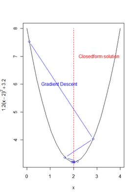
This is minimized by solving for the values of theta that set the derivative to zero. In some cases this can be done analytically with calculus and a little algebra, but this can also be done (especially when complex functions are involved) via gradient descent. Recall from before, the basic gradient descent algorithm involves a learning rate 'alpha' and an update function that utilizes the 1st derivitive or gradient f'(.). The basic algorithm is as follows:

repeat until convergence {
  x := x - α∇F(x) 
}

(see here for a basic demo using R code)

For the case of OLS, and the cost function J(theta) depicted above, the gradient descent algorithm can be implemented in pseudo-code as follows:


It turns out that:


and the gradient descent algorithm becomes:


The following R -Code implements this algorithm and achieves the same results we got from the matrix programming or the canned R or SAS routines before. The concept of 'feature scaling' is introduced, which is a method of standardizing the independent variables or features. This improves the convergence speed of the algorithm. Additional code intuitively investigates the concept of convergence. Ideally, the algorithm should stop once changes in the cost function become small as we update the values in theta.

R-Code:

#  ----------------------------------------------------------------------------------
# |PROGRAM NAME: gradient_descent_OLS_R
# |DATE: 11/27/11
# |CREATED BY: MATT BOGARD 
# |PROJECT FILE:              
# |----------------------------------------------------------------------------------
# | PURPOSE: illustration of gradient descent algorithm applied to OLS
# | REFERENCE: adapted from : http://www.cs.colostate.edu/~anderson/cs545/Lectures/week6day2/week6day2.pdf                
# |  and http://www.statalgo.com/2011/10/17/stanford-ml-1-2-gradient-descent/
#  ---------------------------------------------------------------------------------
 
# get data 
rm(list = ls(all = TRUE)) # make sure previous work is clear
ls()
x0 <- c(1,1,1,1,1) # column of 1's
x1 <- c(1,2,3,4,5) # original x-values
 
# create the x- matrix of explanatory variables
 
x <- as.matrix(cbind(x0,x1))
 
# create the y-matrix of dependent variables
 
y <- as.matrix(c(3,7,5,11,14))
m <- nrow(y)
 
# implement feature scaling
x.scaled <- x
x.scaled[,2] <- (x[,2] - mean(x[,2]))/sd(x[,2])
 
# analytical results with matrix algebra
 solve(t(x)%*%x)%*%t(x)%*%y # w/o feature scaling
 solve(t(x.scaled)%*%x.scaled)%*%t(x.scaled)%*%y # w/ feature scaling
 
# results using canned lm function match results above
summary(lm(y ~ x[, 2])) # w/o feature scaling
summary(lm(y ~ x.scaled[, 2])) # w/feature scaling
 
# define the gradient function dJ/dtheata: 1/m * (h(x)-y))*x where h(x) = x*theta
# in matrix form this is as follows:
grad <- function(x, y, theta) {
  gradient <- (1/m)* (t(x) %*% ((x %*% t(theta)) - y))
  return(t(gradient))
}
 
# define gradient descent update algorithm
grad.descent <- function(x, maxit){
    theta <- matrix(c(0, 0), nrow=1) # Initialize the parameters
 
    alpha = .05 # set learning rate
    for (i in 1:maxit) {
      theta <- theta - alpha  * grad(x, y, theta)   
    }
 return(theta)
}
 
 
# results without feature scaling
print(grad.descent(x,1000))
 
# results with feature scaling
print(grad.descent(x.scaled,1000))
 
# ----------------------------------------------------------------------- 
# cost and convergence intuition
# -----------------------------------------------------------------------
 
# typically we would iterate the algorithm above until the 
# change in the cost function (as a result of the updated b0 and b1 values)
# was extremely small value 'c'. C would be referred to as the set 'convergence'
# criteria. If C is not met after a given # of iterations, you can increase the
# iterations or change the learning rate 'alpha' to speed up convergence
 
# get results from gradient descent
beta <- grad.descent(x,1000)
 
# define the 'hypothesis function'
h <- function(xi,b0,b1) {
 b0 + b1 * xi 
}
 
# define the cost function   
cost <- t(mat.or.vec(1,m))
  for(i in 1:m) {
    cost[i,1] <-  (1 /(2*m)) * (h(x[i,2],beta[1,1],beta[1,2])- y[i,])^2 
  }
 
totalCost <- colSums(cost)
print(totalCost)
 
# save this as Cost1000
cost1000 <- totalCost
 
# change iterations to 1001 and compute cost1001
beta <- (grad.descent(x,1001))
cost <- t(mat.or.vec(1,m))
  for(i in 1:m) {
    cost[i,1] <-  (1 /(2*m)) * (h(x[i,2],beta[1,1],beta[1,2])- y[i,])^2 
  }
cost1001 <- colSums(cost)
 
# does this difference meet your convergence criteria? 
print(cost1000 - cost1001)
Created by Pretty R at inside-R.org

Basic Econometrics in R and SAS

Regression Basics

y= b0 + b1 *X  ‘regression line we want to fit’

The method of least squares minimizes the squared distance between the line ‘y’ and
individual data observations yi


That is minimize: ∑ ei2 = ∑ (yi - b0 -  b1 Xi )2   with respect to b0 and  b1 .
This can be accomplished by taking the partial derivatives of  ∑ ei2 with respect to each coefficient and setting it equal to zero.
∂ ∑ ei2 / ∂ b0 =  2 ∑ (yi - b0 -  b1 Xi )  (-1) = 0 
∂ ∑ ei2 / ∂ b1 =   2 ∑(yi - b0 -  b1 Xi )  (-Xi) = 0
Solving for b0 and  b1 yields the ‘formulas’ for hand calculating the estimates:
b0 = ybar - b1 Xbar
b1 = ∑ (( Xi - Xbar)  (yi - ybar)) / ∑ ( Xi - Xbar) =  [ ∑Xi Yi  – n xbar*ybar] / [∑X2 – n Xbar2
 =   S( X,y) / SS(X)
 
Example with Real Data: 

Given real data, we can use the formulas above to derive (by hand /caclulator/excel) the estimated values for b0 and b1, which give us the line of best fit, minimizing  ∑ ei2 = ∑ (yi - b0 -  b1 Xi )2  .

n= 5
∑Xi Yi   = 146
∑X2  = 55
Xbar = 3
Ybar =8

b1 =  [ ∑Xi Yi  – n xbar*ybar] / [∑X2 – n Xbar2]    (146-5*3*8)/(55-5*32) = 26/10 = 2.6
b0= ybar - b1 Xbar  = 8-2.6*3 = .20

You can verify these results in PROC REG in SAS.

/* GENEARATE DATA */

DATA REGDAT;
INPUT X Y;
CARDS;
1 3
2 7
3 5
4 11
5 14
;
RUN;

/* BASIC REGRESSION WITH PROC REG */

PROC REG DATA = REGDAT;
MODEL Y = X;
RUN;
QUIT;

OUTPUT:


Similarly this can be done in R using the 'lm' function:

#------------------------------------------------------------
#  regression with canned lm routine
#------------------------------------------------------------
 
# read in data manually
 
x <- c(1,2,3,4,5) # read in x -values
 
y <- c(3,7,5,11,14) # read in y-values
 
data1 <- data.frame(x,y) # create data set combining x and y values
 
# analysis
 
plot(data1$x, data1$y) # plot data 
reg1 <- lm(data1$y~data1$x) # compute regression estimates
summary(reg1)              # print regression output
abline(reg1)               # plot fitted regression line
Created by Pretty R at inside-R.org

 
Regression Matrices

Alternatively, this problem can be represented in matrix format. 
We can then formulate the least squares equation as:
 y = Xb 
   
where the ‘errors’  or deviations from the fitted line can be formulated by the matrix :
e = (y – Xb)

The matrix equivalent of ∑ ei2  becomes (y - Xb)’ (y - Xb) = e’e

= (y - Xb)’ (y - Xb) = y’y - 2 * b’X’y + b’X’Xb

Taking partials, setting = 0, and solving for  b   gives:

d e’e / d b = -2 * X’y +2* X’Xb = 0

2 X’Xb =   2 X’y

X’Xb = X’y

b = (X’X)-1  X’y   which is the matrix equivalent to what we had before:
[ ∑Xi Yi  – n xbar*ybar] / [∑X2 – n Xbar2]  =   S( X,y) / SS(X)
 These computations can be carried out in SAS via PROC IML commands:

/* MATRIX REGRESSION */

PROC IML;

/* INPUT DATA AS VECTORS */
yt = {3 7 5 11 14} ; /* TRANSPOSED Y VECTOR */
x0t = j(1,5,1); /* ROW VECTOR OF 1'S */
x1t = {1 2 3 4 5}; /* X VALUES */
xt =x0t//x1t; /* COMBINE VECTORS INTO TRANSPOSED X-MATRIX */

PRINT yt x0t x1t;

/* FORMULATE REGRESSION MATRICES */

y= yt`;     /* VECTOR OF DEPENDENT VARIABLES */
x =xt`; /* FULL X OR DESIGN MATRIX */
beta = inv(x`*x)*x`*y;  /* THE CLASSICAL REGRESSION MATRIX */
PRINT beta;
TITLE 'REGRESSION MATRICES VIA PROC IML';
QUIT;
RUN;

OUTPUT
The same results can be obtained in R as follows:
#------------------------------------------------------------
#   matrix programming based approach
#------------------------------------------------------------
 
# regression matrices require a column of 1's in order to calculate 
# the intercept or constant, create this column of 1's as x0
 
x0 <- c(1,1,1,1,1) # column of 1's
x1 <- c(1,2,3,4,5) # original x-values
 
# create the x- matrix of explanatory variables
 
x <- as.matrix(cbind(x0,x1))
 
# create the y-matrix of dependent variables
 
y <- as.matrix(c(3,7,5,11,14))
 
# estimate  b = (X'X)^-1 X'y
 
b <- solve(t(x)%*%x)%*%t(x)%*%y
 
print(b) # this gives the intercept and slope - matching exactly 
         # the results above
Created by Pretty R at inside-R.org

Gradient Descent in R

In a previous post I discussed the concept of gradient descent.  Given some recent work in the online machine learning course offered at Stanford,  I'm going to extend that discussion with an actual example using R-code  (the actual code is adapted from a computer science course at Colorado State, and the example is verbatim from the notes here: http://www.cs.colostate.edu/~anderson/cs545/Lectures/week6day2/week6day2.pdf )

Suppose you want to minimize the function 1.2 * (x-2)^2 + 3.2. Basic calculus requires that we find the 1st derivative and solve for the value of x such that f'(x) = 0. This is easy enough to do, f'(x) = 2*1.2*(x-2). Its easy to see that a value of 2 satisfies f'(x) =  0. Given that the second order conditions hold, this is a minimum.

Its not alwasys the case that we would get a function so easy to work with, and in many cases we may need to numerically estimate the value that minimizes the function. Gradient descent offers a way to do this. Recall from my previous post the gradient descent algorithm can be summarized as follows:

repeat until convergence {
Xn+1 = Xn - α∇F(Xn)  or  x := x - α∇F(x)  (depending on your notational preferences)
}

Where ∇F(x)  would be the derivative we calculated above for the function at hand and α is the learning rate. This can easily be implemented R. The following code finds the values of x that minimize the function above and plots the progress of the algorithm with each iteration. (as depicted in the image below)


R-code:
#  ----------------------------------------------------------------------------------
# |PROGRAM NAME: gradient_descent_R
# |DATE: 11/27/11
# |CREATED BY: MATT BOGARD 
# |PROJECT FILE:              
# |----------------------------------------------------------------------------------
# | PURPOSE: illustration of gradient descent algorithm
# | REFERENCE: adapted from : http://www.cs.colostate.edu/~anderson/cs545/Lectures/week6day2/week6day2.pdf                
# | 
#  ---------------------------------------------------------------------------------
 
xs <- seq(0,4,len=20) # create some values
 
# define the function we want to optimize
 
f <-  function(x) {
1.2 * (x-2)^2 + 3.2
}
 
# plot the function 
plot(xs , f (xs), type="l",xlab="x",ylab=expression(1.2(x-2)^2 +3.2))
 
# calculate the gradeint df/dx
 
grad <- function(x){
  1.2*2*(x-2)
}
 
 
# df/dx = 2.4(x-2), if x = 2 then 2.4(2-2) = 0
# The actual solution we will approximate with gradeint descent
# is  x = 2 as depicted in the plot below
 
lines (c (2,2), c (3,8), col="red",lty=2)
text (2.1,7, "Closedform solution",col="red",pos=4)
 
 
# gradient descent implementation
x <- 0.1 # initialize the first guess for x-value
xtrace <- x # store x -values for graphing purposes (initial)
ftrace <- f(x) # store y-values (function evaluated at x) for graphing purposes (initial)
stepFactor <- 0.6 # learning rate 'alpha'
for (step in 1:100) {
x <- x - stepFactor*grad(x) # gradient descent update
xtrace <- c(xtrace,x) # update for graph
ftrace <- c(ftrace,f(x)) # update for graph
}
 
lines ( xtrace , ftrace , type="b",col="blue")
text (0.5,6, "Gradient Descent",col="blue",pos= 4)
 
# print final value of x
print(x) # x converges to 2.0
Created by Pretty R at inside-R.org

Monday, November 21, 2011

Revenue and Outlays 1980-1989

As the visualization indicates, revenues grew during the 1980's after cuts in marginal income tax rates, while spending also increased outpacing revenues and driving deficits.
The default charts were produced from default output (html and flash) generated by the R-code that follows.

I added one tweak, as described in the google visualization documentation here:
http://code.google.com/apis/chart/interactive/docs/gallery/motionchart.html which essentially saves the modifications to the settings in the chart. For more info regarding the data format, see my earlier post here.

Note- there are 3 visualization options - bubbles, dynamic bar chart, and a static line graph . These can be selected using the tabs at the top of the graph.

Created Using R- GoogleVis Package
Flash Enable Browser Required!


Data: budget • Chart ID: MotionChartID32de6867
R version 2.13.1 (2011-07-08) • googleVis-0.2.11
Google Terms of UseData Policy

We also saw patterns of increasing revenues during the Bush years following cuts in marginal tax rates, and a period from 2003-2007 where revenues were increasing and deficits were falling.  After the financial crisis, notice how revenues plunged while the deficit exploded.

Revenues and Outlays 2003-2009

(if preloaded labels and settings are not immediately applied, please use direct link for this post here.)


The data source is the CBO Budget/Historical Tables. I'd provide a link but it moves around constantly. A Google search should direct you to the most recent data.

R-Code:(for the first visualization)

#  ----------------------------------------------------------------------------------
# |PROGRAM NAME: budget_vis_R
# |DATE: 11/21/11
# |CREATED BY: MATT BOGARD 
# |PROJECT FILE:              
# |----------------------------------------------------------------------------------
# | PURPOSE: visualization of revenues and outlays in relation to 
# |          cuts in marginal tax rates 1980-89        
# | 
#  ---------------------------------------------------------------------------------
 
# see http://stackoverflow.com/questions/4646779/embedding-googlevis-charts-into-a-web-site/4649753#4649753
# for original R code reference
 
install.packages('googleVis') # install package if first time
 
library(googleVis) # load package
 
#  set R working directory- this is where your data file will go
#  with the script for creating the visualization
 
setwd("C:\\Users\\Documents\\Briefcase\\R Code and Data")
 
# read pre-formated  data
 
budget <- read.csv("budget.csv", na.strings=c(".", "NA", "", "?"), encoding="UTF-8")
names(budget)
 
M <- gvisMotionChart(budget, "ITEM","YEAR")
 
#  look at data object- this includes the script that
#  will be used if you want to publish on your web page/blog
 
print(M) 
 
# open your browser and display the visualization
 
plot(M)
Created by Pretty R at inside-R.org

Thursday, November 10, 2011

Singular Value Decomposition and Text Mining

Single Value Decomposition (SVD) is a concept from linear algebra based on the following matrix equation:
A = USV which states that a rectangular matrix A can be decomposed into 3 other matrix components:

U  consists of the orthonormal eigenvectors of AA’,  where U’U =  I (recall from linear algebra, orthogonal vectors of unit length are ‘orthonormal’)
V consists of the orthonormal eigenvectors of A’A
S  is a diagonal matrix consisting of the square root of the eigenvalues of U or V (which are equal). The values in S depict the variance of linearly independent components along each dimension similarly to the way eigenvalues depict variance explained by ‘factors’ or components in principle components analysis (PCA).

(below is an entertaining video depicting SVD)


In relation to text mining, SVD provides the mathematical foundation for text mining and classification techniques generally known as latent semantic indexing. In SVD, the matrix A is typically a word x document matrix, it is a way of representing your document and text as a highly dimensional vector space model, also referred to as hyperspace document representation.  Similarly  to PCA , SVD takes high dimensional highly variable data and reduces it to a lower dimensional space that more clearly depicts the underlying structure of the data.  SVD reduces noise and redundancy in the data leaving you with new dimensions that capture the essence of existing relationships.   With regard to text mining, SVD has the following interpretation:

-documents are represented as rows in V
-document similarity can be determined by examining rows in VS
- words are represented as rows in U
- word similarity can be determined by examining the rows in the matrix US

References:

SAS Text Miner: Theory and Practice at UnitedHealthcare
Mark Pitts and Chris Clark, UnitedHealthcare (Presentation at Analytics 2011 Conference)

Singular Value Decomposition Tutorial. Kirk Baker. March 29, 2005. http://www.cs.wits.ac.za/~michael/SVDTut.pdf