Remarks from Literature:
‘The basic idea of Bayesian Model Averaging (BMA) is to make inferences based on a weighted average over model space.’ (Hoeting*)
‘BMA accounts for uncertainty in (an) estimated logistic regression by taking a weighted average of the maximum likelihood estimates produced by our models…and may be superior to stepwise regression’ ( Goenner and Pauls, 2006)
‘The uniform prior ( which assumes that each of the K models is equally likely)… is typical in cases that lack strong prior beliefs.’ (Goenner and Pauls, 2006 and Raftery 1995).
References:
Goenner , Cullen F. and Kenton Pauls. ‘A Predictive Model of Inquiry to Enrollment.’ Research in Higher Education, Vol 47, No 8, December 2006.
*Jennifer A. Hoeting, Colorado State Univeristy. ‘Methodology for Bayesian Model Averaging: An Update’
Hoeting, Madigan, Reftery, and Volinksy. ‘ Bayesian Model Averaging: A Tutorial.’ Statistical Science 1999, Vol 14, No 4, 382-417.
Peter Kennedy. ‘A Guide to Econometrics.’ 5th Edition. 2003 MIT Press
Raftery, Madian and Hoeting. ‘Bayesian Model Averaging for Linear Regression Models.’ Journal of the American Statistical Association (1997) 92, 179-191
Raftery A.E. ‘Bayesian Model Selection in Social Research .’ In: Marsden, P.V. (ed): Sociological Methodology 1995, Blackwells Publishers, Cambridge, MA, pp. 111-163.
Studenmund, A.H. Using Econometrics A Practical Guide. 4th Ed. Addison Wesley. 2001
SAS/STAT 9.2 User’s Guide. Introduction to Bayesian Analysis Procedures.
Wednesday, September 22, 2010
Tuesday, September 21, 2010
Path Analysis
PATH ANALYSIS: An application of regression analysis to define connections or paths between variables. Several simultaneous regressions may be specified and can be visualized by a path diagram.
Y1 = b11 X1 + b12 X2+ b13 X3+ + e1
X3 = b21 X1 + b22 X2+ e2
X2 = b31 X1 + e3

Y1 = b11 X1 + b12 X2+ b13 X3+ + e1
X3 = b21 X1 + b22 X2+ e2
X2 = b31 X1 + e3

Partial Least Squares
PARTIAL LEAST SQUARES: For Y = X, derive latent vectors (principle components) of X and Y and use them to explain the covariance of X and Y.


Monday, September 20, 2010
Why study Applied/Agricultural Economics?
Why study Applied/Agricultural Economics? (for an updated post on this topic see here.)
"The combination of quantitative training and applied work makes agricultural economics graduates an extremely well-prepared source of employees for private industry. That's why American Express has hired over 80 agricultural economists since 1990." - David Edwards, Vice President-International Risk Management, American Express
Applied Economics is a broad field covering many topics beyond those stereotypically thought of as pertaining to agriculture. These may include finance and risk management, environmental and natural resource economics, behavioral economics, game theory, or public policy analysis to name a few. More and more 'Agricultural Economics' is becoming synonymous with 'Applied Economics.' Many departments have changed their name from Agricultural Economics to Agricultural and Applied Economics and some have even changed their degree program names to just 'Applied Economics.' In 2008, the American Agricultural Economics Association changed its name to the Agricultural and Applied Economics Association.
This trend is noted in recent research in the journal Applied Economic Perspectives and Policy:
"Increased work in areas such as agribusiness, rural development, and environmental economics is making it more difficult to maintain one umbrella organization or to use the title “agricultural economist” ... the number of departments named" Agricultural Economics” has fallen from 36 in 1956 to 9 in 2007."
Agricultural/Applied economics provides students with skills in high demand, particularly in the area of analytics.
"Some companies have built their very business on their ability to collect, analyze, and act on data." (See 'Competing on Analytics." Harvard Bus.Review Jan 2006)
In a recent blog post, SAS (a leader in applied analytics, big data, and software solutions) highlights the fact that they find people with applied economics backgrounds among their exectives:
"computer science may not be the best place to find data scientists....Over the years many of our senior executives have had degrees in agricultural-related disciplines like forestry, agricultural economics, etc."
Recently from the New York Times: (For Today’s Graduate, Just One Word: Statistics )
"Though at the fore, statisticians are only a small part of an army of experts using modern statistical techniques for data analysis. Computing and numerical skills, experts say, matter far more than degrees. So the new data sleuths come from backgrounds like economics, computer science and mathematics."
To quote, from Johns Hopkins University’s applied economics program home page:
“Economic analysis is no longer relegated to academicians and a small number of PhD-trained specialists. Instead, economics has become an increasingly ubiquitous as well as rapidly changing line of inquiry that requires people who are skilled in analyzing and interpreting economic data, and then using it to effect decisions ………Advances in computing and the greater availability of timely data through the Internet have created an arena which demands skilled statistical analysis, guided by economic reasoning and modeling.”
Finally, a quote I found on the (formerly) American Agricultural Economics Association's web page a few years ago:
“Nearly one in five jobs in the United States is in food and fiber production and distribution. Fewer than three percent of the people involved in the agricultural industries actually work on the farm. Graduates in agricultural and applied economics or agribusiness work in a variety of institutions applying their knowledge of economics and business skills related to food production, rural development and natural resources.”
UPDATE: This brief podcast from the University of Minnesota's Department of Applied Economics does a great job covering the breadth of questions and problems applied economists address in their work
https://podcasts.apple.com/mt/podcast/what-is-applied-economics/id419408183?i=1000411492398
UPDATE: See also Economists as Data Scientists http://econometricsense.blogspot.com/2012/10/economists-as-data-scientists.html
References:
'What is the Future of Agricultural Economics Departments and the Agricultural and Applied Economics Association?' By Gregory M. Perry. Applied Economic Perspectives and Policy (2010) volume 32, number 1, pp. 117–134.
'Competing on Analytics.' Harvard Bus.Review Jan 2006
‘For Today’s Graduate, Just One Word: Statistics.’ Steve Lohr. August 5, 2009
Decision Trees
DECISION TREES: 'Classification and Decision Trees'(CART) Divides the training set into rectangles (partitions) based on simple rules and a measure of 'impurity.' (recursive partitioning) Rules and partitions can be visualized as a 'tree.' These rules can then be used to classify new data sets.
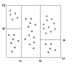
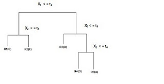
(Adapted from ‘The Elements of Statistical Learning ‘ Hasti, Tibshirani,Friedman)
RANDOM FORESTS: An ensemble of decision trees.
CHI-SQUARED AUTOMATIC INTERACTION DETECTION: characterized by the use of a chi-square test to stop decision tree splits. (CHAID) Requires more computational power than CART.
Neural Networks
NEURAL NETWORK: A nonlinear model of complex relationships composed of multiple 'hidden' layers (similar to composite functions)
Y = f(g(h(x)) or
x -> hidden layers ->Y
Example 1 With a logistic/sigmoidal activation function, a neural network can be visualized as a sum of weighted logits:
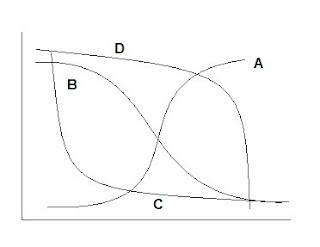
Y = α Σ wi e θi/1 + e θi + ε
wi = weights θ = linear function Xβ
Y= 2 + w1 Logit A + w2 Logit B + w3 Logit C + w4 Logit D
( Adapted from ‘A Guide to Econometrics, Kennedy, 2003)
Example 2

Y = f(g(h(x)) or
x -> hidden layers ->Y

Example 1 With a logistic/sigmoidal activation function, a neural network can be visualized as a sum of weighted logits:

Y = α Σ wi e θi/1 + e θi + ε
wi = weights θ = linear function Xβ
Y= 2 + w1 Logit A + w2 Logit B + w3 Logit C + w4 Logit D
( Adapted from ‘A Guide to Econometrics, Kennedy, 2003)
Example 2

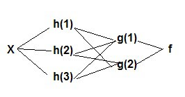
Where: Y= W0 + W1 Logit H1 + W2 Logit H2 + W3 Logit H3 + W4 Logit H4 and
H1= logit(w10 +w11 x1 + w12 x2 )
H2 = logit(w20 +w21 x1 + w22 x2 )
H3 = logit(w30 +w31 x1 + w32 x2 )
H4 = logit(w40 +w41 x1 + w42 x2 )


The links between each layer in the diagram correspond to the weights (w’s) in each equation. The weights can be estimated via back propagation.
( Adapted from ‘A Guide to Econometrics, Kennedy, 2003 and Applied Analytics Using SAS Enterprise Miner 6.1)
MULTILAYER PERCEPTRON: a neural network architecture that has one or more hidden layers, specifically having linear combination functions in the hidden and output layers, and sigmoidal activation functions in the hidden layers. (note: a basic logistic regression function can be visualized as a single layer perceptron)
RADIAL BASIS FUNCTION (architecture): a neural network architecture with exponential or softmax (generalized multinomial logistic) activation functions and radial basis combination functions in the hidden layers and linear combination functions in the output layers.
RADIAL BASIS FUNCTION: A combination function that is based on the Euclidean distance between inputs and weights
ACTIVATION FUNCTION: formula used for transforming values from inputs and the outputs in a neural network.
COMBINATION FUNCTION: formula used for combining transformed values from activation functions in neural networks.
HIDDEN LAYER: The layer between input and output layers in a neural network.
HIDDEN LAYER: The layer between input and output layers in a neural network.
Data Mining in A Nutshell
# The following code may look rough, but simply paste into R or
# a text editor (especially Notepad++) and it will look
# much better.
# PROGRAM NAME: MACHINE_LEARNING_R
# DATE: 4/19/2010
# AUTHOR : MATT BOGARD
# PURPOSE: BASIC EXAMPLES OF MACHINE LEARNING IMPLEMENTATIONS IN R
# DATA USED: GENERATED VIA SIMULATION IN PROGRAM
# COMMENTS: CODE ADAPTED FROM : Joshua Reich (josh@i2pi.com) April 2, 2009
# SUPPORT VECTOR MACHINE CODE ALSO BASED ON :
# ëSupport Vector Machines in Rî Journal of Statistical Software April 2006 Vol 15 Issue 9
#
# CONTENTS: SUPPORT VECTOR MACHINES
# DECISION TREES
# NEURAL NETWORK
# load packages
library(rpart)
library(MASS)
library(class)
library(e1071)
# get data
# A simple function for producing n random samples
# from a multivariate normal distribution with mean mu
# and covariance matrix sigma
rmulnorm <- function (n, mu, sigma) {
M <- t(chol(sigma))
d <- nrow(sigma)
Z <- matrix(rnorm(d*n),d,n)
t(M %*% Z + mu)
}
# Produce a confusion matrix
# there is a potential bug in here if columns are tied for ordering
cm <- function (actual, predicted)
{
t<-table(predicted,actual)
t[apply(t,2,function(c) order(-c)[1]),]
}
# Total number of observations
N <- 1000 * 3# Number of training observations
Ntrain <- N * 0.7 # The data that we will be using for the demonstration consists
# of a mixture of 3 multivariate normal distributions. The goal
# is to come up with a classification system that can tell us,
# given a pair of coordinates, from which distribution the data
# arises.
A <- rmulnorm (N/3, c(1,1), matrix(c(4,-6,-6,18), 2,2))
B <- rmulnorm (N/3, c(8,1), matrix(c(1,0,0,1), 2,2))
C <- rmulnorm (N/3, c(3,8), matrix(c(4,0.5,0.5,2), 2,2))
data <- data.frame(rbind (A,B,C))
colnames(data) <- c('x', 'y')
data$class <- c(rep('A', N/3), rep('B', N/3), rep('C', N/3))
# Lets have a look
plot_it <- function () {plot (data[,1:2], type='n')
points(A, pch='A', col='red')
points(B, pch='B', col='blue')
points(C, pch='C', col='orange')
}
plot_it()

# Randomly arrange the data and divide it into a training
# and test set.
data <- data[sample(1:N),]train <- data[1:Ntrain,]
test <- data[(Ntrain+1):N,]
# SVM
# Support vector machines take the next step from LDA/QDA. However
# instead of making linear voronoi boundaries between the cluster
# means, we concern ourselves primarily with the points on the
# boundaries between the clusters. These boundary points define
# the 'support vector'. Between two completely separable clusters
# there are two support vectors and a margin of empty space
# between them. The SVM optimization technique seeks to maximize
# the margin by choosing a hyperplane between the support vectors
# of the opposing clusters. For non-separable clusters, a slack
# constraint is added to allow for a small number of points to
# lie inside the margin space. The Cost parameter defines how
# to choose the optimal classifier given the presence of points
# inside the margin. Using the kernel trick (see Mercer's theorem)
# we can get around the requirement for linear separation
# by representing the mapping from the linear feature space to
# some other non-linear space that maximizes separation. Normally
# a kernel would be used to define this mapping, but with the
# kernel trick, we can represent this kernel as a dot product.
# In the end, we don't even have to define the transform between
# spaces, only the dot product distance metric. This leaves
# this algorithm much the same, but with the addition of
# parameters that define this metric. The default kernel used
# is a radial kernel, similar to the kernel defined in my
# kernel method example. The addition is a term, gamma, to
# add a regularization term to weight the importance of distance.
s <- svm( I(factor(class)) ~ x + y, data = train, cost = 100, gama = 1)
s # print model results
#plot model and classification-my code not originally part of this
plot(s,test)

(m <- cm(train$class, predict(s)))
1 - sum(diag(m)) / sum(m)
(m <- cm(test$class, predict(s, test[,1:2])))
1 - sum(diag(m)) / sum(m)
# Recursive Partitioning / Regression Trees
# rpart() implements an algorithm that attempts to recursively split
# the data such that each split best partitions the space according
# to the classification. In a simple one-dimensional case with binary
# classification, the first split will occur at the point on the line
# where there is the biggest difference between the proportion of
# cases on either side of that point. The algorithm continues to
# split the space until a stopping condition is reached. Once the
# tree of splits is produced it can be pruned using regularization
# parameters that seek to ameliorate overfitting.
names(train)names(test)
(r <- rpart(class ~ x + y, data = train)) plot(r) text(r) summary(r) plotcp(r) printcp(r) rsq.rpart(r)

cat("\nTEST DATA Error Matrix - Counts\n\n")
print(table(predict(r, test, type="class"),test$class, dnn=c("Predicted", "Actual")))
# Here we look at the confusion matrix and overall error rate from applying
# the tree rules to the training data.
predicted <- as.numeric(apply(predict(r), 1, function(r) order(-r)[1]))
(m <- cm (train$class, predicted))
1 - sum(diag(m)) / sum(m)
# Neural Network
# Recall from the heuristic on data mining and machine learning , a neural network is # a nonlinear model of complex relationships composed of multiple 'hidden' layers
# (similar to composite functions)
# Build the NNet model.
require(nnet, quietly=TRUE)
crs_nnet <- nnet(as.factor(class) ~ ., data=train, size=10, skip=TRUE, trace=FALSE, maxit=1000)
# Print the results of the modelling.
print(crs_nnet)
print("
Network Weights:
")
print(summary(crs_nnet))
# Evaluate Model Performance
# Generate an Error Matrix for the Neural Net model.
# Obtain the response from the Neural Net model.
crs_pr <- predict(crs_nnet, train, type="class")
# Now generate the error matrix.
table(crs_pr, train$class, dnn=c("Predicted", "Actual"))
# Generate error matrix showing percentages.
round(100*table(crs_pr, train$class, dnn=c("Predicted", "Actual"))/length(crs_pr))
Calucate overall error percentage.
print( "Overall Error Rate")
(function(x){ if (nrow(x) == 2) cat((x[1,2]+x[2,1])/sum(x)) else cat(1-(x[1,rownames(x)])/sum(x))}) (table(crs_pr, train$class, dnn=c("Predicted", "Actual")))
Sunday, September 19, 2010
Logistic Modeling & Maximum Likelihood Estimation vs. Linear Regression & Ordinary Least Squares
See also: Analysis of the Logistic Function
Ordinary Least Squares:
OLS: y = XB + e
Minimizes the sum of squared residuals e'e where e = (y –XB)
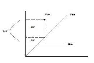
R2 = 1- SSE/SST
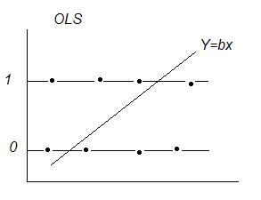
OLS With a Dichotomous Dependent Variable: y = (0 or 1)
Dichotomous Variables, Expected Value, & Probability:
Linear Regression E[y|X] = XB ‘conditional mean(y) given x‘
If y = { 0 or 1}
E[y|X] = Pi a probability interpretation
Expected Value: sum of products of each possible value a variable can take * the probability of that value occurring.
If P(y=1) = pi and P(y=0) = (1-pi) then E[y] = 1*pi +0* (1-pi) = pi → the probability that y=1
Problems with OLS:
1) Estimated probabilities outside (0,1)
2) e~binomial var(e) = n*p*(1-p) violates assumption of uniform variance → unreliable inferences
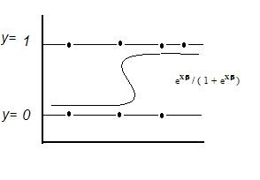
Logit Model:
Ln ((Di /(1 – Di)) = βX
Di = probability y = 1 = eXβ / ( 1 + eXβ )
Where : Di / (1 – Di) = ’odds’
E[y|X] = Prob(y = 1|X) = p = eXβ / (1 + eXβ )
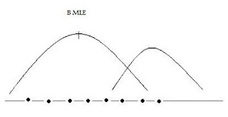
Maximum Likelihood Estimation
L(θ) =∏f(y,θ) -the product of marginal densities
Take ln of both sides, choose θ to maximize, → θ* (MLE)
Choose θ’s to maximize the likelihood of the sample being observed.Maximizes the likelihood that data comes from a ‘real world’ characterized by one set of θ’s vs another.
Estimating a Logit Model Using Maximum Likelihood:
L(β) = ∏f(y, β) = ∏ eXβ / (1 + eXβ ) ∏ 1/(1 + eXβ)
choose β to maximize the ln(L(β)) to get the MLE estimator β*
To get p(y=1) apply the formula Prob( y = 1|X) = p = eXβ* / (1 + eXβ*) utilizing the MLE estimator β*to'score' the data X.
Deriving Odds Ratios:
Exponentiation ( eβ ) gives the odds ratio.
Variance:
When we undertake MLE we typically maximize the log of the likelihood function as follows:
Max Log(L(β)) or LL ‘log likelihood’ or solve:
∂Log(L(β))/∂β = 0 'score matrix' = u( β)
-∂u(β)/ ∂β 'information matrix' = I(β)
Inference:
√W ~ t or Z (based on assumptions exact or asymptotic normality)
Assessing Model Fit and Predictive Ability:
Not minimizing sums of squares: R2 = 1 – SSE / SST or SSR/SST. With MLE no sums of squares are produced and no direct measure of R2 is possible. Other measures must be used to assess model performance:
-2[LL0 - LL1] L0 = likelihood of incomplete model L1 = likelihood of more complete model
Model Deviance: DK = -2[LLK - LLp] LK = intercept only model Lp= perfect model ~ SSR
Model χ2 : DN -DK For a good fitting model, model deviance will be smaller than null deviance, giving a larger χ2 and a higher level of significance.
Pseudo-r-square: DN -DK / DN Smaller (better fitting) DK gives a larger ratio. Not on (0,1)
Cox & Snell Pseudo R square: adjusts for parameters and sample size, not on (0,1)
Nagelkerke (Max-rescaled r-square) : transformation such that R --> (0,1)
Other:
Percentage of Correct Predictions
Area under the ROC curve:
Area = measure of model’s ability to correctly distinguish cases where (y=1) from those that do not based on explanatory variables.
y-axis: sensitivity or prediction that y = 1 when y = 1,
x-axis: 1-specificity or prediction that y = 1 when y = 0, false positive
References:
Menard, Applied Logistic Regression Analysis, 2nd Edition 2002
Ordinary Least Squares:
OLS: y = XB + e
Minimizes the sum of squared residuals e'e where e = (y –XB)
R2 = 1- SSE/SST

OLS With a Dichotomous Dependent Variable: y = (0 or 1)

Dichotomous Variables, Expected Value, & Probability:
Linear Regression E[y|X] = XB ‘conditional mean(y) given x‘
If y = { 0 or 1}
E[y|X] = Pi a probability interpretation
Expected Value: sum of products of each possible value a variable can take * the probability of that value occurring.
If P(y=1) = pi and P(y=0) = (1-pi) then E[y] = 1*pi +0* (1-pi) = pi → the probability that y=1
Problems with OLS:
1) Estimated probabilities outside (0,1)
2) e~binomial var(e) = n*p*(1-p) violates assumption of uniform variance → unreliable inferences
Logit Model:
Ln ((Di /(1 – Di)) = βX
Di = probability y = 1 = eXβ / ( 1 + eXβ )
Where : Di / (1 – Di) = ’odds’
E[y|X] = Prob(y = 1|X) = p = eXβ / (1 + eXβ )

Maximum Likelihood Estimation
L(θ) =∏f(y,θ) -the product of marginal densities
Take ln of both sides, choose θ to maximize, → θ* (MLE)
Choose θ’s to maximize the likelihood of the sample being observed.Maximizes the likelihood that data comes from a ‘real world’ characterized by one set of θ’s vs another.

Estimating a Logit Model Using Maximum Likelihood:
L(β) = ∏f(y, β) = ∏ eXβ / (1 + eXβ ) ∏ 1/(1 + eXβ)
choose β to maximize the ln(L(β)) to get the MLE estimator β*
To get p(y=1) apply the formula Prob( y = 1|X) = p = eXβ* / (1 + eXβ*) utilizing the MLE estimator β*to'score' the data X.
Deriving Odds Ratios:
Exponentiation ( eβ ) gives the odds ratio.
Variance:
When we undertake MLE we typically maximize the log of the likelihood function as follows:
Max Log(L(β)) or LL ‘log likelihood’ or solve:
∂Log(L(β))/∂β = 0 'score matrix' = u( β)
-∂u(β)/ ∂β 'information matrix' = I(β)
I-1 (β) 'variance-covariance matrix' = cramer rao lower bound
Inference:
Wald χ2 = (βMLE -β0)Var-1(βMLE -β0)
Assessing Model Fit and Predictive Ability:
Not minimizing sums of squares: R2 = 1 – SSE / SST or SSR/SST. With MLE no sums of squares are produced and no direct measure of R2 is possible. Other measures must be used to assess model performance:
Deviance: -2 LL where LL = log-likelihood (smaller is better)
-2[LL0 - LL1] L0 = likelihood of incomplete model L1 = likelihood of more complete model
AIC and SC are deviants of -2LL, and penalize the LL by the # of predictors in the model
Null Deviance: DN = -2[LLN - LLp] LN = intercept only model Lp= perfect model ~ SST
Model Deviance: DK = -2[LLK - LLp] LK = intercept only model Lp= perfect model ~ SSR
Model χ2 : DN -DK For a good fitting model, model deviance will be smaller than null deviance, giving a larger χ2 and a higher level of significance.
Pseudo-r-square: DN -DK / DN Smaller (better fitting) DK gives a larger ratio. Not on (0,1)
Cox & Snell Pseudo R square: adjusts for parameters and sample size, not on (0,1)
Nagelkerke (Max-rescaled r-square) : transformation such that R --> (0,1)
Other:
Percentage of Correct Predictions
Area under the ROC curve:

Area = measure of model’s ability to correctly distinguish cases where (y=1) from those that do not based on explanatory variables.
y-axis: sensitivity or prediction that y = 1 when y = 1,
x-axis: 1-specificity or prediction that y = 1 when y = 0, false positive
References:
Menard, Applied Logistic Regression Analysis, 2nd Edition 2002
Support Vector Machines
Separates classes utilizing supporting hyperplanes and a separating hyperplane that maximizes the margin between classes.
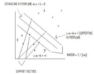
Max 2/||w|| s.t. y(x*w+b)-1 >=0
If data is not linearly separable, a kernel function can be used to map data into a space where it is linearly separable.
Input Space →Kernel Function →Feature Space →Input Space.
Quadratic programming provides a decision function:
D(x) = ∑ ∝ k(xi,xj) + b such that if D(x) >0 then x ∊ A
Kernel Functions
Mapping function x→φ(x)
linear kernel
k(xi,xj)=xi'xj
radial basis kernel
k(xi,xj) = exp[-(||xi –xj||2 / 2 σ2 )]
polynomial kernel
k(xi,xj) = (xixj + a)b
sigmoidal kernel
k(xi ,xj) = tanh(xixj - b)
Spatial Econometrics
OLS: Review
y= Xb + e
Minimize e’e, e = (y-Xb)
b = (X’X)-1 X’y
Generalized Least Squares: A Review
y = Xb + u
u = a vector of random errors with mean 0 and var-cov matrix C
b = (X’ C-1 X)-1X’C-1 y
Geographically Weighted Regression
y = X b(t) + e
b(t) = (X’ W X)-1 X’Wy or Dy
W = spatial weight matrix , which may reflect contiguity between observations, or distance between observations
Spatial Lag Model
y = p Wy + e p = spatial autoregression parameter estimated from the data
Spatial lag Model (Mixed)
y = Xb + p Wy + e
Spatial Error Model
y = Xb + e where e = λ W e + u and u= y – Xb
y = Xb + λ W (y – Xb) + u
= Xb +λ Wy - λ WXb + u
Moran's I: test for spatial autocorrelation
I =(N S)(e'We/e'e)
e = OLS residuals and S = ΣΣ w
References:
Anselin, Luc. ‘Spatial Econometrics.’ Bruton Center. School of Social Sciences. University of Texas. Richardson, TX 75083-0688. http://www.csiss.org/learning_resources/content/papers/baltchap.pdf
Geographically Weighted Regression: The Analysis of Spatially Varying Relationships. A. Stewart Fotheringham et al. Wiley 2002.
George Casella and Edward I. George ‘Explaining the Gibbs Sampler’ The American Statistician, Vol. 46, No. 3, (Aug., 1992), pp. 167-174 American Statistical Association
Geospatial Analysis: A Comprehensive Guide. 2nd edition © 2006-2008 de Smith, Goodchild, Longley
http://www.spatialanalysisonline.com/output/
Rao, C. R. (1973). Linear Statistical Inference and its Applications (2nd Ed.). Wiley, New York.
Tiefelsdorf, Michael. ‘Modeling Spatial Processes: The Identification and Analysis of Spatial Relationships in Regression Residuals by Means of Moran’s I.’ Springer –Verlag Berlin Heidelber 2000. Germany
Symbol Pallete
These can be used to cut and paste in blogger for blog posts:
α β γ δ ε ζ η θ ι κ λ μ ν ξ ο π ρ ς σ τ υ φ χ ψ ω . . . . . Γ Δ Θ Λ Ξ Π Σ Φ Ψ Ω
∂ ∫ ∏ ∑ . . . . . ← → ↓ ↑ ↔ . . . . . ± − · × ÷ √ . . . . . ¼ ½ ¾ ⅛ ⅜ ⅝ ⅞
∞ ° ² ³ ⁿ Å . . . . . ~ ≈ ≠ ≡ ≤ ≥ « » . . . . . † ‼
More:
Source: http://xahlee.blogspot.com/2010/06/math-symbols-in-unicode.html
Some Greeks: α β γ δ ε ζ η θ ι κ λ μ ν ξ ο π ρ ς τ υ φ χ ψ ω
superscript: ⁰ ⁱ ² ³ ⁴ ⁵ ⁶ ⁷ ⁸ ⁹ ⁺ ⁻ ⁼ ⁽ ⁾ ⁿ
subscript: ₀ ₁ ₂ ₃ ₄ ₅ ₆ ₇ ₈ ₉ ₊ ₋ ₌ ₍ ₎ ₐ ₑ ₒ ₓ ₔ
Roots: √ ∛ ∜
Sets: ℕ ℤ ℚ ℝ ℂ
Constants: ℯ ℵ ⅇ ⅈ ⅉ ∅ ∞ ⧜ ⧝ ⧞
Basic binary operators: × ÷ ⊕ ⊖ ⊗ ⊘ ⊙ ⊚ ⊛ ⊜ ⊝ ⊞ ⊟ ⊠ ⊡ − ∕ ∗ ∘ ∙ ⋅ ⋆
Sets
element of: ∈ ∋ ∉ ∌ ⋶ ⋽ ⋲ ⋺ ⋳ ⋻
misc: ∊ ∍ ⋷ ⋾ ⋴ ⋼ ⋵ ⋸ ⋹ ⫙ ⟒
binary relation of sets: ⊂ ⊃ ⊆ ⊇ ⊈ ⊉ ⊊ ⊋ ⊄ ⊅ ⫅ ⫆ ⫋ ⫌ ⫃ ⫄ ⫇ ⫈ ⫉ ⫊ ⟃ ⟄ ⫏ ⫐ ⫑ ⫒ ⫓ ⫔ ⫕ ⫖ ⫗ ⫘ ⋐ ⋑ ⟈ ⟉
Union: ∪ ⩁ ⩂ ⩅ ⩌ ⩏ ⩐
Intersection: ∩ ⩀ ⩃ ⩄ ⩍ ⩎
Binary operator on sets: ∖ ⩆ ⩇ ⩈ ⩉ ⩊ ⩋ ⪽ ⪾ ⪿ ⫀ ⫁ ⫂ ⋒ ⋓
N-nary operator on sets: ⋂ ⋃ ⊌ ⊍ ⊎
Joins: ⨝ ⟕ ⟖ ⟗
Order
Precede and succeed: ≺ ≻ ≼ ≽ ≾ ≿ ⊀ ⊁ ⋞ ⋟ ⋠ ⋡ ⋨ ⋩ ⪯ ⪰ ⪱ ⪲ ⪳ ⪴ ⪵ ⪶ ⪷ ⪸ ⪹ ⪺ ⪻ ⪼
less and greater: ≮ ≯ ≤ ≥ ≰ ≱ ⪇ ⪈ ≦ ≧ ≨ ≩
less and greater 2: ⋜ ⋝ ⪙ ⪚ ≶ ≷ ≸ ≹ ⋚ ⋛ ⪋ ⪌ ⪑ ⪒ ⪓ ⪔
with approx: ⪅ ⪆ ⪉ ⪊
less and greater with equivalence: ≲ ≳ ⋦ ⋧ ≴ ≵
less and greater with similarity: ⪝ ⪞ ⪟ ⪠ ⪍ ⪎ ⪏ ⪐
less and greater slanted: ⩽ ⩾ ⫹ ⫺ ⪕ ⪖ ⪛ ⪜
less and greater misc: ⪣ ⪤ ⪥ ⪦ ⪧ ⪨ ⪩ ⪪ ⪫ ⪬ ⪭ ⪮ ⪡ ⪢ ⫷ ⫸ ⩹ ⩺ ⩻ ⩼ ≬ ≪ ≫ ⋘ ⋙
Order relation with dot: ⋖ ⋗ ⩿ ⪀ ⪗ ⪘ ⪁ ⪂ ⪃ ⪄
Equality, Identity, Equivalence, Approx, Congruence
equality: ≝ ≞ ≟ ≠ ∹ ≎ ≏ ≐ ≑ ≒ ≓ ≔ ≕ ≖ ≗ ≘ ≙ ≚ ≛ ≜ ⩬ ⩭ ⩮ ⩱ ⩲ ⩦ ⩴ ⩵ ⩶ ⩷
Identity: ≡ ≢ ⩧
Equivalence: ≍ ≭ ≣ ⩸
Approx equality: ≁ ≂ ≃ ≄ ⋍ ≅ ≆ ≇ ≈ ≉ ≊ ≋ ≌ ⩯ ⩰
Misc equality: ∻
Misc relations: ⊏ ⊐ ⊑ ⊒ ⊓ ⊔ ⋢ ⋣ ⋤ ⋥ ⊲ ⊳ ⊴ ⊵ ⋪ ⋫ ⋬ ⋭ ⫴ ⫵
Logic
Logic: ¬ ⫬ ⫭ ⊨ ⊭ ∀ ∁ ∃ ∄ ∴ ∵ ⊦ ⊬ ⊧ ⊩ ⊮ ⊫ ⊯ ⊪ ⊰ ⊱
Logic binary: ∧ ∨ ⊻ ⊼ ⊽ ⋎ ⋏ ⟑ ⟇ ⩑ ⩒ ⩓ ⩔ ⩕ ⩖ ⩗ ⩘ ⩙ ⩚ ⩛ ⩜ ⩝ ⩞ ⩟ ⩠ ⩢ ⩣ ⨇ ⨈
Logic n-nary: ⋀ ⋁
n-nary operators: ∑ ⨀ ⨁ ⨂ ⨃ ⨄ ⨅ ⨆ ∏ ∐ ∔
Geometry
Geometry: ∣ ∤ ⫮ ⌅ ⌆ ℓ ⫛
Ratio and proportion: ∝ ∶ ∷ ∺
Parallel and perpendicular: ∥ ∦ ⫲ ⫳ ⋕ ⟂ ⫡
Right angle: ∟ ⊾ ⦜ ⦝ ⊿
Angles: ∠ ∡ ⦛ ⦞ ⦟ ⦢ ⦣ ⦤ ⦥ ⦦ ⦧ ⦨ ⦩ ⦪ ⦫ ⦬ ⦭ ⦮ ⦯ ⦓ ⦔ ⦕ ⦖ ⟀
Spherical angle: ∢ ⦠ ⦡
...
Pairs: ⌈ ⌉ ⌊ ⌋ ⦋ ⦌ ⟦ ⟧ ⦍ ⦎ ⦏ ⦐
pairs 2: ⟮ ⟯ ⟨ ⟩ ⟪ ⟫ ⦃ ⦄ ⦅ ⦆ ⦇ ⦈ ⦉ ⦊ ⟬ ⟭ ⦗ ⦘ ⦑ ⦒ ⧼ ⧽
integrals: ∫ ∬ ∭ ∮ ∯ ∰ ∱ ∲ ∳ ⨋ ⨌ ⨍ ⨎ ⨏ ⨐ ⨑ ⨒ ⨓ ⨔ ⨕ ⨖ ⨗ ⨘ ⨙ ⨚ ⨛ ⨜
Derivative: ∂ ′ ″ ‴ ∆
vector: ⨯ ∇ ⊹
Misc indicators: ∎ ± ∓ ⋮ ⋯ ⋰ ⋱
Misc symbols: ∿
Tacks: ⊣ ⊢ ⊥ ⊤ ⟘ ⟙ ⟛ ⟝ ⟞ ⟟ ⫧ ⫨ ⫩ ⫪ ⫫ ⫞ ⫟ ⫠
Turnstiles: ⫢ ⫣ ⫤ ⫥ ⟚
Z notation: ⦁ ⦂ ⩤ ⩥ ⨟ ⨠ ⨡ ⨾
Tilde Operators: ∼ ∽ ⩪ ⩫ ⩳
Misc Operators: ⋄ ⫶ ⫼ ⫾
Misc products: ≀ ⨿ ⨼ ⨽ ⧢ ⋉ ⋊ ⋋ ⋌
Plus variations: ⨢ ⨣ ⨤ ⨥ ⨦ ⨧ ⨨ ⨭ ⨮
Solidus: ⫻ ⫽
minus sign variations: ∸ ⨩ ⨪ ⨫ ⨬
maps: ⊶ ⊷ ⊸ ⟜ ⧟
Saturday, September 18, 2010
Using R
By Matt Bogard
Abstract
R is a statistical programming language with a command line interface that is becoming more and more popular every day. I have used R for data visualization, data mining/machine learning, as well as social network analysis. Initially embraced largely in academia, R is becoming the software of choice in various corporate settings.
Download in pdf
Overview of Concepts in Data Mining and Machine Learning
BAGGING: Acronym for ‘bootstrap aggregating.’ A technique that relies on sampling with replacement. By taking a number N of bootstrap samples, N models are fit, one from each sample. For regression, the models are combined or averaged. For classification 'votes' or outcomes from each model are tallied with the majority determining a given class.
BOOSTING: Developing an 'ensemble' or additive model composed of simple rules or weak learners. These rules are combined in such a way that each ensemble member's performance is improved or 'boosted.'
SUPPORT VECTOR MACHINES: Separates classes utilizing supporting hyperplanes and a separating hyperplane that maximizes the margin between classes.
NEURAL NETWORK: A nonlinear model of complex relationships composed of multiple 'hidden' layers (similar to composite functions)
Y = f(g(h(x)) or
x -> hidden layers ->Y
MULTILAYER PERCEPTRON: a neural network that has one or more hidden layers.
HIDDEN LAYER: The layer between input and output in a neural network, characterized by an activation function.
DECISION TREES: 'Classification and Decision Trees'(CART) Divides the training set into rectangles (partitions) based on simple rules and a measure of 'impurity.' (recursive partitioning) Rules and partitions can be visualized as a 'tree.' These rules can then be used to classify new data sets.
RANDOM FORESTS: An ensemble of decision trees.
CHI-SQUARED AUTOMATIC INTERACTION DETECTION: characterized by the use of a chi-square test to stop decision tree splits. (CHAID) Requires more computational power than CART.
NAÏVE BAYES: Classification based on an application of Bayes Theorem. Referred to as 'naive' because of strong independence assumptions:
P(x…x|c) = P(xi|cj)
(x.....x) values are conditionaly independent given class C.
This technique is useful because it is often more computationally tractable to calculate the probabilities on the right side than the left.
SURVIVAL ANALYSIS: Models the failure time or occurrence of an event. Define a 'survival' function that relates 't' (failure time variable) to Y. Using the survival function, a likelihood function can be specified.
DESCRIMINANT ANALYSIS: Weights are estimated that form a linear function maximizing between group vs. within group variance. Can be visualized as a line that separates groups.
CLUSTER ANALYSIS: Utilizes a measure of distance to define homogeneous clusters or classes of data
K-MEANS CLUSTERING: Defines a centroid or average of all points in a cluster of data. Observations are assigned to the cluster that has the 'nearest' or closest mean value. The space defined by cluster centroids is equivalent to the subspace defined by principal components of the data set.
K-NEAREST NEIGHBOR: an observation takes the same classification as the most common class of its k-nearest neighbors.
K-FOLD CROSS VALIDATION: Models are constructed by training on all but 1 of 'K' subsets of data. This is repeated K-1 times.
MARKET BASKET ANALYSIS-APRIORI ALGORITHM: Derives rules based on the probability of items occurring together. A conditional probability is used as a measure of 'confidence.' Example: The probability that A and C occur together ( A --> C) can be defined as P(A∩B)/P(C) = P(C|A)
LIFT: the increase in the probability of an event given the occurrence of another event. Lift = support/(support(A) + support(C))
PARTIAL LEAST SQUARES: For Y = X, derive latent vectors (principle components) of X and use them to explain the covariance of X and Y.
PATH ANALYSIS: An application of regression analysis to define connections or paths between variables. Several simultaneous regressions may be specified and can be visualized by a path diagram.
STRUCTURAL EQUATION MODELING: Path analysis utilizing latent variables. Combines regression analysis and factor analysis in a simultaneous equation model.
PRINCIPLE COMPONENTS ANALYSIS: Y = Ax The components of A are eigenvectors of an observed covariance matrix S or correlation matrix R. They define principal axis that maximize the variance of a data set. The principal components Y = (y.....y) define new uncorrelated variables that provide an alternative 'reduced' representation of the original data.
FACTOR ANALYSIS: Utilizes principal components analysis to partition total variance into common an unique variance based on underlying factors and assumptions of a statistical model.
X = L F + U
X = observations
L = loadings of X derived from iterations of PCA
F = theoretical factor, defined by the X's that load most heavily on that factor
U = unique variance
GENETIC ALGORITHMS: parallel concepts from genetics to model data. (inheritance,mutaton,selection,crossover)
Friday, September 17, 2010
Data Mining/Machine Learning Overview
For example code in R related to some of these topics see 'Data Mining in A Nutshell' -link
BAGGING: Acronym for ‘bootstrap aggregating.’ A technique that relies on sampling with replacement. By taking a number N of bootstrap samples, N models are fit, one from each sample. For regression, the models are combined or averaged. For classification 'votes' or outcomes from each model are tallied with the majority determining a given class.
BOOSTING: Developing an 'ensemble' or additive model composed of simple rules or weak learners. These rules are combined in such a way that each ensemble member's performance is improved or 'boosted.'
SUPPORT VECTOR MACHINES: Separates classes utilizing supporting hyperplanes and a separating hyperplane that maximizes the margin between classes.
NEURAL NETWORK: A nonlinear model of complex relationships composed of multiple 'hidden' layers (similar to composite functions)
Y = f(g(h(x)) or
x -> hidden layers ->Y
DECISION TREES: 'Classification and Decision Trees'(CART) Divides the training set into rectangles (partitions) based on simple rules and a measure of 'impurity.' (recursive partitioning) Rules and partitions can be visualized as a 'tree.' These rules can then be used to classify new data sets.
RANDOM FORESTS: An ensemble of decision trees.
CHI-SQUARED AUTOMATIC INTERACTION DETECTION: characterized by the use of a chi-square test to stop decision tree splits. (CHAID) Requires more computational power than CART.
NAÏVE BAYES: A generative learning algorithm based on an application of Bayes Theorem. Referred to as 'naive' because of strong independence assumptions:
p(yi|x) = p(x|yi)p(yi) / p(x) 'bayes rule'
p(x|y) = p(x1,x2|y) = p(x1|y) p(x2|y) = ∏ p(xk|yi) 'conditional independence assumption'
SURVIVAL ANALYSIS: Models the failure time or occurrence of an event. Define a 'survival' function that relates 't' (failure time variable) to Y. Using the survival function, a likelihood function can be specified.
DESCRIMINANT ANALYSIS: Weights are estimated that form a linear function maximizing between group vs. within group variance. Can be visualized as a line that separates groups.
CLUSTER ANALYSIS: Utilizes a measure of distance to define homogeneous clusters or classes of data
K-MEANS CLUSTERING: Defines a centroid or average of all points in a cluster of data. Observations are assigned to the cluster that has the 'nearest' or closest mean value. The space defined by cluster centroids is equivalent to the subspace defined by principal components of the data set.
K-NEAREST NEIGHBOR: an observation takes the same classification as the most common class of its k-nearest neighbors.
K-FOLD CROSS VALIDATION: Models are constructed by training on all but 1 of 'K' subsets of data. This is repeated K-1 times.
MARKET BASKET ANALYSIS-APRIORI ALGORITHM: Derives rules based on the probability of items occurring together. A conditional probability is used as a measure of 'confidence.' Example: The probability that A and C occur together ( A --> C) can be defined as P(A∩B)/P(C) = P(CA)
LIFT: the increase in the probability of an event given the occurrence of another event. Lift = support/(support(A) + support(C))
PARTIAL LEAST SQUARES: For Y = X, derive latent vectors (principle components) of X and use them to explain the covariance of X and Y.
PATH ANALYSIS: An application of regression analysis to define connections or paths between variables. Several simultaneous regressions may be specified and can be visualized by a path diagram.
STRUCTURAL EQUATION MODELING: Path analysis utilizing latent variables. Combines regression analysis and factor analysis in a simultaneous equation model.
PRINCIPLE COMPONENTS ANALYSIS: Y = Ax The components of A are eigenvectors of an observed covariance matrix S or correlation matrix R. They define principal axis that maximize the variance of a data set. The principal components Y = (y.....y) define new uncorrelated variables that provide an alternative 'reduced' representation of the original data.
FACTOR ANALYSIS: Utilizes principal components analysis to partition total variance into common an unique variance based on underlying factors and assumptions of a statistical model.
X = L F + U
X = observations
L = loadings of X derived from iterations of PCA
F = theoretical factor, defined by the X's that load most heavily on that factor
U = unique variance
GENETIC ALGORITHMS: Analogizes concepts from genetics to model data in an iterative multistep (multigenerational) process.
Each ‘generation’ is a completion of 5 steps, iterating for 3-5 generations generates estimators.
1) Chromosomes = S initial random samples
2) Fitness = predictive accuracy
3) Replicate chromosomes weighting by fitness
4) Crossover = randomly select 2 chromosomes to form 2 new ‘recombinants’
5) Mutations = initiate random changes in randomly selected chromosomes
BAGGING: Acronym for ‘bootstrap aggregating.’ A technique that relies on sampling with replacement. By taking a number N of bootstrap samples, N models are fit, one from each sample. For regression, the models are combined or averaged. For classification 'votes' or outcomes from each model are tallied with the majority determining a given class.
BOOSTING: Developing an 'ensemble' or additive model composed of simple rules or weak learners. These rules are combined in such a way that each ensemble member's performance is improved or 'boosted.'
SUPPORT VECTOR MACHINES: Separates classes utilizing supporting hyperplanes and a separating hyperplane that maximizes the margin between classes.
NEURAL NETWORK: A nonlinear model of complex relationships composed of multiple 'hidden' layers (similar to composite functions)
Y = f(g(h(x)) or
x -> hidden layers ->Y
DECISION TREES: 'Classification and Decision Trees'(CART) Divides the training set into rectangles (partitions) based on simple rules and a measure of 'impurity.' (recursive partitioning) Rules and partitions can be visualized as a 'tree.' These rules can then be used to classify new data sets.
RANDOM FORESTS: An ensemble of decision trees.
CHI-SQUARED AUTOMATIC INTERACTION DETECTION: characterized by the use of a chi-square test to stop decision tree splits. (CHAID) Requires more computational power than CART.
NAÏVE BAYES: A generative learning algorithm based on an application of Bayes Theorem. Referred to as 'naive' because of strong independence assumptions:
p(yi|x) = p(x|yi)p(yi) / p(x) 'bayes rule'
p(x|y) = p(x1,x2|y) = p(x1|y) p(x2|y) = ∏ p(xk|yi) 'conditional independence assumption'
p(yi|x) = ∏ p(xk|yi) p(yi) / p(x) 'naive bayes'
DESCRIMINANT ANALYSIS: Weights are estimated that form a linear function maximizing between group vs. within group variance. Can be visualized as a line that separates groups.
CLUSTER ANALYSIS: Utilizes a measure of distance to define homogeneous clusters or classes of data
K-MEANS CLUSTERING: Defines a centroid or average of all points in a cluster of data. Observations are assigned to the cluster that has the 'nearest' or closest mean value. The space defined by cluster centroids is equivalent to the subspace defined by principal components of the data set.
K-NEAREST NEIGHBOR: an observation takes the same classification as the most common class of its k-nearest neighbors.
K-FOLD CROSS VALIDATION: Models are constructed by training on all but 1 of 'K' subsets of data. This is repeated K-1 times.
MARKET BASKET ANALYSIS-APRIORI ALGORITHM: Derives rules based on the probability of items occurring together. A conditional probability is used as a measure of 'confidence.' Example: The probability that A and C occur together ( A --> C) can be defined as P(A∩B)/P(C) = P(CA)
LIFT: the increase in the probability of an event given the occurrence of another event. Lift = support/(support(A) + support(C))
PARTIAL LEAST SQUARES: For Y = X, derive latent vectors (principle components) of X and use them to explain the covariance of X and Y.
PATH ANALYSIS: An application of regression analysis to define connections or paths between variables. Several simultaneous regressions may be specified and can be visualized by a path diagram.
STRUCTURAL EQUATION MODELING: Path analysis utilizing latent variables. Combines regression analysis and factor analysis in a simultaneous equation model.
PRINCIPLE COMPONENTS ANALYSIS: Y = Ax The components of A are eigenvectors of an observed covariance matrix S or correlation matrix R. They define principal axis that maximize the variance of a data set. The principal components Y = (y.....y) define new uncorrelated variables that provide an alternative 'reduced' representation of the original data.
FACTOR ANALYSIS: Utilizes principal components analysis to partition total variance into common an unique variance based on underlying factors and assumptions of a statistical model.
X = L F + U
X = observations
L = loadings of X derived from iterations of PCA
F = theoretical factor, defined by the X's that load most heavily on that factor
U = unique variance
GENETIC ALGORITHMS: Analogizes concepts from genetics to model data in an iterative multistep (multigenerational) process.
Each ‘generation’ is a completion of 5 steps, iterating for 3-5 generations generates estimators.
1) Chromosomes = S initial random samples
2) Fitness = predictive accuracy
3) Replicate chromosomes weighting by fitness
4) Crossover = randomly select 2 chromosomes to form 2 new ‘recombinants’
5) Mutations = initiate random changes in randomly selected chromosomes
Mathematical Themes in Economics, Machine Learning and Bioinformatics
By Matt Bogard
Abstract
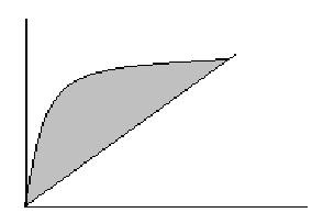
Graduate students in economics are often introduced to some very useful mathematical tools that many outside the discipline may not associate with training in economics. This essay looks at some of these tools and concepts, including constrained optimization, separating hyperplanes, supporting hyperplanes, and ‘duality.’ Applications of these tools are explored including topics from machine learning and bioinformatics.
Download Full Text
Abstract
Graduate students in economics are often introduced to some very useful mathematical tools that many outside the discipline may not associate with training in economics. This essay looks at some of these tools and concepts, including constrained optimization, separating hyperplanes, supporting hyperplanes, and ‘duality.’ Applications of these tools are explored including topics from machine learning and bioinformatics.
Download Full Text
A. Concepts from Mathematical Statistics
Probability Density Functions
Random Variables
A random variable takes on values that have specific probabilities of occurring. An example of a random variable would be the number of car accidents per year among sixteen year olds. If we know how random variables are distributed in a population, then we may have an idea of how rare an observation may be. This information is then useful for making inferences (or drawing conclusions) about the population of random variables by using sample data.
Example Random Variable: How often sixteen year olds are involved in auto accidents in a year’s time.
Application: We could look at a sample of data consisting of 1,000 sixteen year olds in the Midwest and make inferences or draw conclusions about the population consisting of all sixteen year olds in the Midwest.
In summary, it is important to be able to specify how a random variable is distributed. It enables us to gauge how rare an observation (or sample) is and then gives us ground to make predictions, or inferences about the population.
Random variables can be discrete, that is observed in whole units as in counting numbers 1,2,3,4 etc. Random variables may also be continuous. In this case random variables can take on an infinite number of values. An example would be crop yields. Yields can be measured in bushels down to a fraction or decimal. The distributions of discrete random variables can be presented in tabular form or with histograms. Probability is represented by the area of a ‘rectangle’ in a histogram
Distributions for continuous random variables cannot be represented in tabular format due to their characteristic of taking on an infinite number of values. They are better represented by a smooth curve defined by a function. This function is referred to as a probability density function or p.d.f.
The p.d.f. gives the probability that a random variable ‘X’ takes on values in a narrow interval ‘dx’. This probability is equivalent to the area under the (p.d.f.) curve. This area can be described by the cumulative density function c.d.f. This can be obtained through integration of the p.d.f. over a given range.
Let f(x) be a p.d.f.
P( a <= X <= b ) = a∫b f(x) dx = F ( x )
This can be interpreted to mean that the probability that X is between the values of ‘a’ and ‘b’ is given by the integral of the p.d.f from ‘a’ to ‘b.’ This value can be given by the c.d.f. which is F ( x ). Those familiar with calculus know that F(x) is the anti-derivative of f(x).
f(x)= 1 / (2π σ ) -1/2 e –1/2 (x - u )^2/ sigma2
where X~ N ( u, σ2 )
In the beginning of this section I stated that it was important to be able to specify how a random variable is distributed. Through experience, statisticians have found that they are justified in modeling many random variables with these p.d.f.’s. Therefore, in many cases one can be justified in using one of these p.d.f.’s to determine how rare a sample observation is, and then to make inferences about the population. This is in fact what takes place when you look up values from the tables in the back of statistics textbooks.
Mathematical Expectation
The expected value E(X) for a discrete random variable can be determined by adding the products of individual observations Xi multiplied by the probability of observing each Xi .The expected value of an observation is the mean of a distribution of observations. It can be thought of conceptually as an average or weighted mean.
Example: given the p.d.f. for the discrete random variable X in tabular format.
Xi : 1 2 3
P(x =xi) .25 .50 .25
E (X) = SUM Xi P(x =xi) = 1 * .25 + 2*.50 + 3*.25 = 2.0
...to be conitued
Subscribe to:
Posts (Atom)