Mediators and Moderators

Moderators: With moderation, a third variable impacts or interacts with the relationship between two other variables. We would say the relationship between two variables is ‘moderated.’ This can be thought of as an interaction in a standard regression:

Y = b0 + b1*X1 + b2*X2 + b3*X1*X2

b3 =moderating effect i.e. the relationship between Y and X1 changes with levels of X2
b1 = impact of X1 on Y when X2 = 0.

So in the context of the relationship between Y and X1, X2 is a moderator

Mediators: With mediation, a third variable invervenes in the relationship between two other variables. For example, in the diagram below, suppose we are interested in the relationship between x and y. This relationship may be ‘mediated’ by a third variable m.

Consider a model where Y = grade in course (our outcome of interest), k = IQ, m =  study skills. We might hypothesize that study skills ‘mediate’ the effect of IQ on course grade. A perfectly brilliant person might do OK on an exam through educated guesses, but we all might know of cases where brilliant students have done quite poor due to lax study skills. So while there may be a direct effect of IQ on grades, IQ -> grades or x -> y there is an indirect effect as well, IQ->Study Skills -> grade or x -> m -> y.

This implies that mediation can take a number of forms and can be formally tested. In the case of full mediation, the relationship between x and y becomes insignificant after a mediator ‘m’ is included in the model, or our estimate of c (modeling the path or direct effect between x and y) isn’t significantly different from 0. Partial mediation would occur if the relationship between x and y or  c is reduced (but remains significant) after m is entered into the model).  In this case we could say that x has both direct effects on y (through the path c) as well as an indirect effect (through the mediator m or paths a and b).

These relationships can be formally tested as laid out in Hair et al:

1) Test for significant correlations between x,y or estimate c; x,m or estimate a; m,y or estimate b
2) If c is significant after m is included, and the magnitude of c does not change then m is not a mediator.
3) If the magnitude of c is reduced after including m, and c remains significant, then m is a moderator. This is a case of partial mediation.
4) If including m in the model reduces the magnitude of c such that it is not significantly different from 0, then m is a mediator and this is considered a case of full mediation.

Reference: Multivariate Data Analysis. 6th Edition. Harris, Black, Babin, Anderson and Tatham. Pearson-Prentice Hall. 2006.

How is it that Structural Equation Models Subsume Potential Outcomes?

I have been trying to figure out, under what conditions can we identify causal effects via SEMs, particularly, is there a framework similar to the Rubin Causal Model or potential outcomes framework that I can utilize in this attempt?  In search of an answer I ran across the following article:

Comments and Controversies
Cloak and DAG: A response to the comments on our comment
Martin A. Lindquist, Michael E. Sobel
Neuroimage. 2013 Aug 1;76:446-9

On potential outcomes notation:

"Personally, we find that using this notation helps us to formulate problems clearly and avoid making mistakes, to understand and develop identification conditions for estimating causal effects, and, very importantly, to discuss whether or not such conditions are plausible or implausible in practice (as above). Though quite intuitive, the notation requires a little getting used to, primarily because it is not typically included in early statistical training, but once that is accomplished, the notation is powerful and simple to use. Finally, as a strictly pragmatic matter, the important papers in the literature on causal inference (see especially papers by the 3R's (Robins, Rosenbaum, Rubin, and selected collaborators)) use this notation, making an understanding of it a prerequisite for any neuroimaging researcher who wants to learn more about this subject."

The notation definitely takes a little time getting use to, and it is also true for me that it was not discussed early on in any of my biostatistics or econometrics courses. However, Angrist and Pischke's Mostly Harmless Econometrics does a good job making it more intuitive, with a little effort.  Pearl and Bollen both make arguments that SEMs 'subsume' the potential outcomes framework.While this may be true, its not straightforward to me yet. But I agree it is important to understand how SEMs relate to potential outcomes and causality, or at least understand some framework to support their use in causal inference, as stated in the article:

"Our original note had two aims. First, we wanted neuroimaging researchers to recognize that when they use SEMs to make causal inferences, the validity of the conclusions rest on assumptions above and beyond those required to use an SEM for descriptive or predictive purposes. Unfortunately, these assumptions are rarely made explicit, and in many instances, researchers are not even aware that they are needed. Since these assumptions can have a major impact on the “finndings”, it is critical that researchers be aware of them, and even though they may not be testable, that they think carefully about the science behind their problem and utilize their substantive knowledge to carefully consider, before using an SEM, whether or not these assumptions are plausible in the particular problem under consideration."

I think the assumptions they provide 1-4b seem to lay a foundation in terms that make sense to me from a potential outcomes framework, and the authors hold that these are the assumptions one should think about before using SEMs for causal inference.

Perceptions of GMO Foods: A Hypothetical Application of SEM

Suppose we were interested in understanding consumer perceptions of GMO foods. People often make decisions and form opinions about issues based on abstract constructs like fears, goals, ambitions, values, political ideology etc. These are things that may not be so easy to quantify, despite being relevant to behavior and choice. When it comes to perceptions of GMO food, perhaps they are shaped by some degree of skepticism of ‘big ag’ or chemical companies. We could call this ‘monsantophobia.’ Perceptions of biotechnology could also be shaped by the extent of one’s knowledge of basic biology, agricultural science, and genetics.  This second construct could be referred to as a ‘science’ factor. A third ‘factor’ that may shape one’s views could be based on their ideals related to the role of government and political ideology. We’ll call this the ‘political’ factor.

So how can we best quantify these ‘latent’ constructs or ‘factors’ that may be related to perceptions of biotechnology, and how do we model these interactions?  This will require a combination of techniques involving factor analysis and regression, known as structural equation modeling. We might administer a survey, asking key questions that relate to one’s level of monsantophobia,  science knowledge, and political views.  To the extend that ‘monsantophobia’ exists and shapes views on biotechnology, it should flavor responses  to questions related to fears, skepticism, and mistrust of ‘big ag.’ Actual knowledge of science should influence responses to questions related to science etc. We also may want to quantify the actual flavor of perceptions of GMO food. This could be some index quantifying levels of tolerance or preferences related to policies concerning labeling, testing, and regulation or purchasing decisions and expenditures on related goods.  To the extent that perceptions are ‘positive’ the index would reflect that on some scale related to answers to survey questions about these issues. You could also include a set of questions related to policy preferences and try to model the interaction of the above factors and their impact on the support for some policy or the general policy environment.

Suppose we ask a range of questions related to skepticism of big ag and agrochemical companies and record the responses to each question as a value for a number of variables (X_m1…X_mn), and did the same for science knowledge (X_s1…X_sn), political ideology (X_p1…X_pn), and overall GMO perception (Y_p1…Y_pn) and policy environment (Y_e1…Y_en) . Given the values of these variables will be influenced by the actual latent constructs we are trying to measure, we refer to the X’s and Y’s above as ‘indicators’ of the given factors for monsantophobia, science, politics, gmo perception, and policy environment. They may also be referred to as the observable manifest variables.

Now, this is not a perfect system of measurement.  Given the level of subjectivity among other things, there is likely to be a non-negligible amount of measurement error involved.  How can we deal with measurement error and quantify the factors? Factor analysis attempts to separate common variance (associated with the factors) from unique variance in a data set. Theoretically, the unique variance in FA is correlated with the measurement error we are concerned about, while the factors remain ‘uncontaminated’ (Dunteman,1989).

Structural equation modeling (SEM) consists of two models, a measurement model which consists of deriving the latent constructs or factors previously discussed, and a structural model, which relates the factors to one another, and possibly some outcome. In this case, we are relating the factors related to monsantophobia, science, and political preferences to the outcome, which in this case would be the latent construct or index related to GMO perceptions and policy environment. By using the measured ‘factors’ from FA, we can quantify the latent constructs of monsantophobia, science, politics ,and GMO perceptions with less measurement error than if we simply included the numeric responses for the X’s and Y’s in a normal regression.  And then SEM lets us identify the relative influence of each of these factors on GMO perceptions and perhaps even their impact on the general policy environment for biotechnology. This is done in a way similar to regression, by estimating path coeffceints for the paths connecting the latent constructs or factors as depicted below.

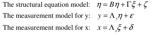
Equations:

References:

Principle Components Analysis- SAGE Series on Quantitative  Applcations in the Social Sciences. Dunteman. 1989.

Awareness and Attitudes towards Biotechnology Innovations among Farmers and Rural Population in the European Union
LUIZA TOMA1, LÍVIA MARIA COSTA MADUREIRA2, CLARE HALL1, ANDREW BARNES1, ALAN RENWICK1

Paper prepared for presentation at the 131st EAAE Seminar ‘Innovation for Agricultural Competitiveness and Sustainability of Rural Areas’, Prague, Czech Republic, September 18-19, 2012

A Structural Equation Model of Farmers Operating within Nitrate Vulnerable Zones (NVZ) in Scotland
Toma, L.1, Barnes, A.1, Willock, J.2, Hall, C.1
12th Congress of the European Association of Agricultural Economists – EAAE 2008

PLoS One. 2014; 9(1): e86174.
Published online Jan 29, 2014. doi:  10.1371/journal.pone.0086174
PMCID: PMC3906022
Determinants of Public Attitudes to Genetically Modified Salmon
Latifah Amin,1,* Md. Abul Kalam Azad,1,2 Mohd Hanafy Gausmian,3 and Faizah Zulkifli1