Logistic Modeling & Maximum Likelihood Estimation vs. Linear Regression & Ordinary Least Squares

See also: Analysis of the Logistic Function 

Ordinary Least Squares:

OLS: y = XB + e

Minimizes the sum of squared residuals e'e where e = (y –XB)

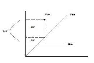
R² = 1- SSE/SST



OLS With a Dichotomous Dependent Variable: y = (0 or 1)



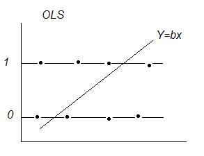
Dichotomous Variables, Expected Value, & Probability:


Linear Regression E[y|X] = XB ‘conditional mean(y) given x‘

If y = { 0 or 1}

E[y|X] = P_i a probability interpretation


Expected Value: sum of products of each possible value a variable can take * the probability of that value occurring.

If P(y=1) = p_i and P(y=0) = (1-p_i) then E[y] = 1*p_i +0* (1-p_i) = p_i → the probability that y=1

Problems with OLS:
1) Estimated probabilities outside (0,1)
2) e~binomial var(e) = n*p*(1-p) violates assumption of uniform variance → unreliable inferences

Logit Model:

Ln ((D_i /(1 – D_i)) = βX

D_i = probability y = 1 = e^Xβ / ( 1 + e^Xβ )

Where : D_i / (1 – D_i) =  ’odds’

E[y|X] = Prob(y = 1|X) = p = e^Xβ / (1 + e^Xβ )



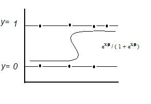
Maximum Likelihood Estimation

L(θ) =∏f(y,θ) -the product of marginal densities
Take ln of both sides, choose θ to maximize, → θ* (MLE)

Choose θ’s to maximize the likelihood of the sample being observed.Maximizes the likelihood that data comes from a ‘real world’ characterized by one set of θ’s vs another.



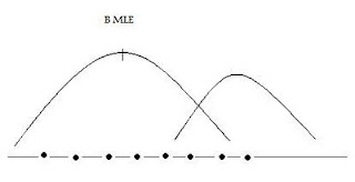
Estimating a Logit Model Using Maximum Likelihood:

L(β) = ∏f(y, β) = ∏ e^Xβ / (1 + e^Xβ ) ∏ 1/(1 + e^Xβ)

choose β to maximize the ln(L(β)) to get the MLE estimator β*

To get p(y=1) apply the formula Prob( y = 1|X) = p = e^Xβ* / (1 + e^Xβ*) utilizing the MLE estimator β*to'score' the data X.

Deriving Odds Ratios:

Exponentiation ( e^β ) gives the odds ratio.

Variance:

When we undertake MLE we typically maximize the log of the likelihood function as follows:

Max Log(L(β)) or LL ‘log likelihood’ or solve:

∂Log(L(β))/∂β = 0     'score matrix'   = u( β)

-∂u(β)/ ∂β    'information matrix'   = I(β)

I^-1 (β)   'variance-covariance matrix'   = cramer rao lower bound

  
Inference:

Wald  χ²  = (β^MLE  -β₀)Var^-1(β^MLE  -β₀)

√W ~ t or Z (based on assumptions exact or asymptotic normality)

Assessing Model Fit and Predictive Ability:

Not minimizing sums of squares: R² = 1 – SSE / SST or SSR/SST. With MLE no sums of squares are produced and no direct measure of R² is possible. Other measures must be used to assess model performance:

Deviance:   -2 LL where   LL = log-likelihood   (smaller is better)  

 -2[LL₀  - LL₁]   L₀  = likelihood of  incomplete model  L₁ =  likelihood  of more complete model

AIC and SC are deviants of -2LL, and penalize the LL by the # of predictors in the model

Null Deviance:  D_N = -2[LL_N  - LL_p]  L_N  = intercept only model  L_p= perfect model ~ SST

Model Deviance: D_K = -2[LL_K  - LL_p]  L_K  = intercept only model  L_p= perfect model ~ SSR

Model χ² : D_N -D_K For a good fitting model, model deviance will be smaller than null deviance, giving a larger χ² and a higher level of significance. 

Pseudo-r-square:   D_N -D_K / D_N  Smaller (better fitting) D_K gives a larger ratio. Not on (0,1)

Cox & Snell Pseudo R square: adjusts for parameters and sample size, not on (0,1)

Nagelkerke (Max-rescaled r-square) :  transformation such that R --> (0,1)

Other: 

Percentage of Correct Predictions

Area under the ROC curve:




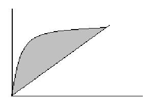
Area = measure of model’s ability to correctly distinguish cases where (y=1) from those that do not based on explanatory variables.

y-axis: sensitivity or prediction that y = 1 when y = 1,
x-axis: 1-specificity or prediction that y = 1 when y = 0, false positive


References:

Menard, Applied Logistic Regression Analysis, 2nd Edition 2002