What is new and different about difference-in-differences?

Back in 2012 I wrote about the basic 2 x 2 difference in difference analysis (two groups, two time periods). Columbia public health probably has a better introduction. 

The most famous example of an analysis that motivates a 2 x 2 DID analysis is John Snow's 1855 analysis of the cholera epidemic in London:

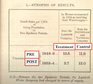
(Image Source)

 I have since written about some of the challenges of estimating DID with glm models (see here, here, and here.), as well as combining DID with matching, and problems to watch out for when combining methods. But a lot of what we know about difference in differences has changed in the last decade. I'll try to give a brief summary based on my understanding and point towards some references that do a better job presenting the current state.

The Two-Way Fixed Effects model (TWFE)

The first thing I should discuss is extending the 2x2 model to include multiple treated groups and/or multiple time periods. The generalized model for DiD also referred to as the two-way fixed effects (TWFE) model is the best way to represent those kind of scenarios:.

Ygt = ag + bt + δDgt + εt

ag = group fixed effects

bt = time fixed effects

Dgt= treatment*post period (interaction term)

δ = ATT or DID estimate

Getting the correct standard errors for DID models that involve many repeated measures over time and/or where treatment and control groups are defined by multiple geographies presents two challenges compared to the basic 2x2 model. Serial correlation and correlation within groups. There are several approaches that can be considered depending on your situation.

1 - Block bootstrapping

2 - Aggregating data into single pre and post periods

3 - Clustering standard errors at the group level

Clustering at the group level should provide the appropriate standard errors in these situations when the number of clusters are large.

For more details on TWFE models, both Scott Cunningham and Nick Huntington-Klein have great econometrics textbooks with chapters devoted to these topics. See the references below for more info.

Differential Timing and Staggered Rollouts

But things can get even more complicated with DID designs. Think about situations where there are different groups getting treated at different times over a number of time periods. This is not just a thought experiment trying to imagine the most difficult study design and pondering for the sake of pondering – these kind of staggered rollouts are very common in business and policy settings.  Imagine policy rules adopted by different states over time (like changes in minimum wages) or imagine testing a new product or service by rolling it out to different markets over time. Understanding how to evaluate their impact is important. For a while it seemed economists may have been a little guilty of handwaving with the TWFE model assuming the estimated treatment coefficient was giving them the effect they wanted. 

But Andrew Goodman-Bacon refused to take this interpretation at face value and broke this down for us determining that the TWFE estimator was trying to give us a weighted average of all potential 2x2 DID estimates you could make with the data. That actually sounds intuitive and helpful. But what he discovered that is not so intuitive is that some of those 2x2 comparisons could be comparing previously treated groups with current treated groups. That's not a comparison we generally are interested in making, but it gets averaged in with the others and can drastically bias the results particularly when there is treatment effect heterogeneity (the treatment effect is different across groups and trending over time). 

So how do you get a better DID estimate in this situation? I'll spare you the details (because I'm still wrestling with them) but the answer seems to be the estimation strategy developed by Callaway and Sant'Anna. The documentation in R for their package walks through a lot of the details and challenges with TWFE models with differential timing. 

Additionally this video of Andrew Goodman-Bacon was really helpful for understanding the 'Bacon' decomposition of TWFE models and the problems above.

After watching Goodman-Bacon, I recommend this talk from Sant'Anna discussing their estimator. 

Below Nick Huntington-Klein provides a great summary of the issues made apparent by the Bacon decomposition made above and the Callaway and Sant'Anna method for staggered/rollout DID designs. he also gets into the Wooldridge Mundlack approach:

A Note About Event Studies

In a number of references I have tried to read to understand this issue, the term 'event study' is thrown around and it seems like every time it is used it is used differently but the author/speaker assumes we are all taking about the same thing. In this video Nick Huntington-Klein introduces event studies in a way that is the most clear and consistent. Watching this video might help.

References: 

Causal Inference: The Mixtape. Scott Cunningham. https://mixtape.scunning.com/ 

The Effect: Nick Huntington-Klein. https://theeffectbook.net/

Andrew Goodman-Bacon. Difference-in-differences with variation in treatment timing. Journal of Econometrics.Volume 225, Issue 2, 2021.

Brantly Callaway, Pedro H.C. Sant’Anna. Difference-in-Differences with multiple time periods. Journal of Econometrics. Volume 225, Issue 2, 2021,

Related Posts:

Modeling Claims Costs with Difference in Differences. https://econometricsense.blogspot.com/2019/01/modeling-claims-with-linear-vs-non.html 

Was It Meant to Be? OR Sometimes Playing Match Maker Can Be a Bad Idea: Matching with Difference-in-Differences. https://econometricsense.blogspot.com/2019/02/was-it-meant-to-be-or-sometimes-playing.html 

Was It Meant to Be? OR Sometimes Playing Match Maker Can Be a Bad Idea: Matching with Difference-in-Differences

Previously I discussed the unique aspects of modeling claims and addressing those with generalized linear models. I followed that with a discussion of the challenges of using difference-in-differences in the context of GLM models and some ways to deal with this. In this post I want to dig into into what some folks are debating in terms of issues related to combining matching with DID. Laura Hatfield covers it well on twitter:

Link: https://twitter.com/laura_tastic/status/1022890688525029376

Do you use diff-in-diff? Then this thread is for you.

You’re no dummy. You already know diverging trends in the pre-period can bias your results.

But I’m here to tell you about a TOTALLY DIFFERENT, SUPER SNEAKY kind of bias.

Friends, let’s talk regression to the mean. (1/N) pic.twitter.com/M2tEEsBiyH

— Laura Hatfield (@laura_tastic) July 27, 2018

Also, they picked up on this it at the incidental economist and gave a good summary of the key papers here.

You can find citations for the relevant papers below. I won't plagerize what both Laura and the folks at the Incidental Economist have already explained very well. But, at a risk of oversimplifying the big picture I'll try to summarize a bit. Matching in a few special cases can improve the precision of the estimate in a DID framework,  and occasionally reduces bias. Remember, that  matching on pre-period observables is not necessary for the validity of difference in difference models. There are  cases when the treatment group is in fact determined by pre-period outcome levels. In these cases matching is necessary. At other times, if not careful, matching in DID introduces risks for regression to the mean…what Laura Hatfield describes as a ‘bounce back’ effect in the post period that can generate or inflate treatment effects when they do not really exist.

Both the previous discussion on DID in a GLM context and combining matching with DID indicate the risks involved in just plug and play causal inference and the challenges of bridging the gap between theory and application.


References:

Daw, J. R. and Hatfield, L. A. (2018), Matching and Regression to the Mean in Difference‐in‐Differences Analysis. Health Serv Res, 53: 4138-4156. doi:10.1111/1475-6773.12993

Daw, J. R. and Hatfield, L. A. (2018), Matching in Difference‐in‐Differences: between a Rock and a Hard Place. Health Serv Res, 53: 4111-4117. doi:10.1111/1475-6773.13017

Modeling Claims with Linear vs. Non-Linear Difference-in-Difference Models

Previously I have discussed the issues with modeling claims costs. Typically medical claims exhibit non-negative highly skewed values with high zero mass and heterskedasticity. The most commonly suggested approach to addressing these distributional concerns in the literature call for the use of non-linear GLM models.  However, as previously discussed (see here and here) there are challenges with using difference-in-difference models in the context of GLM models. So once again, the gap between theory and application presents challenges, tradeoffs, and compromises that need to be made by the applied econometrician.

In the past I have written about the accepted (although controversial in some circles) practice of leveraging linear probability models to estimate marginal effects in applied work when outcomes are dichotomous. But what about doing this in the context of claims analysis? In my original post regarding the challenges of using difference-in-differences with claims I speculated:

"So as Angrist and Pischke might ask, what is an applied guy to do? One approach even in the context of skewed distributions with high mass points (as is common in the healthcare econometrics space) is to specify a linear model. For count outcomes (utilization like ER visits or hospital admissions are often dichotomized and modeled by logit or probit models) you can just use a linear probability model. For skewed distributions with heavy mass points, dichotomization with a LPM may also be an attractive alternative."

 I have found that this advice is pretty consistent with the social norms and practices in the field.

In their analysis of the ACA Cantor, et al (2012) leverage linear probability models for difference-in-differences for healthcare utilization stating:

"Linear probability models are fit to produce coefficients that are direct estimates of the relevant policy impacts and are easily interpreted as percentage point changes in coverage outcomes. This approach has been applied in earlier evaluations of insurance market reforms (Buchmueller and DiNardo 2002; Monheit and Steinberg Schone 2004;  Levine, McKnight, and Heep 2011;  Monheit et al. 2011). It also avoids complications associated with estimation and interpretation of multiple interaction terms and their standard errors in logit or probit models (Ai and Norton 2003)."

Jhamb et al (2015) use LPMs for dichotomous outcomes as well as OLS models for counts in a DID framework.

Interestingly, Deb and Norton (2018) discuss an approach to address the challenges of DID in a GLM framework head on:

"Puhani argued, using the potential outcomes framework, that the treatment effect on the treated in the difference-in-difference regression equals the expected value of the dependent variable for the treatment group in the post period with treatment compared with the hypothetical expected value of the dependent variable for the treatment group in the post period if they had not received treatment. In nonlinear models, the treatment effect on the treated equals the difference in two predicted values. It always has the same sign as the coefficient on the interaction term. Because we estimate many nonlinear models using a difference-in-differences study design, we report the treatment effect on the treated in all tables of results."

In presenting their results they compare their GLM based approach to results from linear models of healthcare expenditures. While they argue the differences are substantial in supporting their approach, I did not find the OLS estimate (-$323.4) to be practically different from the second part (conditional on positive) of the two part GLM model (-$321.4), although the combined results from the two part model had large practical differences from OLS. It does not appear they compared a two-part GLM to a two-part linear model (which could be problematic if the first part OLS model gave probabilities greater than 1 or less than zero). In their paper they cited a number of authors using linear difference-in-differences to model claims you will find below.

See the references below for a number of examples (including those cited above).

Related: Linear Literalism and Fundamentalist Econometrics

References:

Cantor JC, Monheit AC, DeLia D, Lloyd K. Early impact of the Affordable Care Act on health insurance coverage of young adults. Health Serv Res. 2012;47(5):1773-90.

Modeling Health Care Expenditures and Use
Partha Deb and Edward C. Norton
Annual Review of Public Health 2018 39:1, 489-505

Buchmueller T, DiNardo J. “Did Community Rating Induce an Adverse Selection Death Spiral? Evidence from New York, Pennsylvania and Connecticut” American Economic Review. 2002;92(1):280–94.

Monheit AC, Cantor JC, DeLia D, Belloff D. “How Have State Policies to Expand Dependent Coverage Affected the Health Insurance Status of Young Adults?” Health Services Research. 2011;46(1 Pt 2):251–67

Amuedo-Dorantes C, Yaya ME. 2016. The impact of the ACA’s extension of coverage to dependents on young adults’ access to care and prescription drugs. South. Econ. J. 83:25–44

Barbaresco S, Courtemanche CJ, Qi Y. 2015. Impacts of the Affordable Care Act dependent coverage provision on health-related outcomes of young adults. J. Health Econ. 40:54–68

Jhamb J, Dave D, Colman G. 2015. The Patient Protection and Affordable Care Act and the utilization of health care services among young adults. Int. J. Health Econ. Dev. 1:8–25

Sommers BD, Buchmueller T, Decker SL, Carey C, Kronick R. 2013. The Affordable Care Act has led
to significant gains in health insurance and access to care for young adults. Health Aff. 32:165–74

Identification and Common Trend Assumptions in Difference-in-Differences for Linear vs GLM Models

In a previous post I discussed the conclusion from Lechner’s paper 'The Estimation of Causal Effects by Difference-in-Difference Methods', that difference-in-difference models in a non-linear or GLM context failed to meet the common trend assumptions, and therefore failed to identify treatment effects from a selection on unobservables context.

In that post I noted that Lechner points out (quite rigorously in the context of the potential outcomes framework):

"We start with a “natural” nonlinear model with a linear index structure which is transformed by a link function, G(·), to yield the conditional expectation of the potential outcome.....The common trend assumption relies on differencing out specific terms of the unobservable potential outcome, which does not happen in this nonlinear specification... Whereas the linear specification requires the group specific differences to be time constant, the nonlinear specification requires them to be absent. Of course, this property of this nonlinear specification removes the attractive feature that DiD allows for some selection on unobservable group and individual specific differences. Thus, we conclude that estimating a DiD model with the standard specification of a nonlinear model would usually lead to an inconsistent estimator if the standard common trend assumption is upheld. In other words, if the standard DiD assumptions hold, this nonlinear model does not exploit them (it will usually violate them). Therefore, estimation based on this model does not identify the causal effect”

I wanted to review at a high level exactly how he gets to this result. But I wanted to simplify this as much as possible and start with some basic concepts. Starting with a basic regression model, the population conditional expectation function, or conditional mean of Y given X can be written as:

Regression and Expected Value Notation:

E[Y|X] = β₀ + β₁ X (1)

and we estimate this with the regression on observed data:

y = b₀ + b₁X + e (2)

Where b₁ is our estimate of the population parameter of interest β₁.

If E[b₁] = β₁ then we say our estimator is unbiased.

Potential Outcomes Notation:

When it comes to experimental designs, we are interested in knowing counterfactuals, that is what value of an outcome would a treatment or program participant have in absence of treatment (the baseline potential outcome) vs. if they participated or were treated? If we specify these 'potential outcomes' as follows:

Y⁰= baseline potential outcome
Y¹= potential treatment outcome

We can characterize the treatment effect as:

E[Y⁰-Y¹] or the difference in potential treated vs baseline outcomes. This is referred to as the average treatment effect or ATE. Sometimes we are interested in, or some models estimate, the average treatment effect on the treated or ATT :E[Y⁰-Y¹ | d = 1]  

where d is an indicator for treatment (d = 1) vs control or untreated (d =0).

Difference-in-Difference Analysis:

Difference-in-difference (DD) estimators assume that in absence of treatment the difference between control (B) and treatment (A) groups would be constant or ‘fixed’ over time. Treatment effects in DD estimators are derived by subtracting differences between pre and post values within treatment and control groups, and then taking a difference in differences between treatment and control groups. The unobservable effects that are constant or fixed over time 'difference out' allowing us to identify treatment effects controlling for these unobservable characteristics with out explicitly measuring them. This characterizes what is referred to as a 'selection on unobservables' framework.

  This can also be estimated using linear regression with an interaction term:

y = b₀ + b₁ d + b₂ t + b₃ d*t+ e (3)

where d indicates treatment (d=1 vs d = 0) and the estimated coefficient (b₃ ) on the time by treatment interaction term gives us our estimate of treatment effects. 

Lechner and Potential Outcomes Framework:

In an attempt to present the issues with GLM DD models depicted in Lechner (2010) using the simplest notation possible (abusing notation slightly and perhaps at a cost of precision), we can depict the framework for difference-in-difference analysis using expectations:

DID = [E(Y₁|D=1)-E( Y₀|D=1)] -[E(Y₁|D=0)-E(Y₀|D=0)] (4)

DID = [pre/post differences for treatment group] – [pre/post differences for control group]

where Y represents the observed outcome values sub-scripted by pre (0) and post periods(1)

We can represent potential outcomes in the regression framework as follows:

E(Y_t¹|D) = α + tδ¹ + dγ “potential outcome if treated” (5)

E(Y_t⁰|D) = α + tδ⁰ + dγ “potential baseline outcome” (6)

ATET: E(Y_t¹- Y_t⁰|D= 1) = θ₁ = δ    (7)

“difference-in-difference of potential outcomes across time if treated”

We can estimate δ with a regression on observed data of the form:

y = b₀ + b₁ d + b₂ t + b₃ d*t+ e (3')

where b₃ is our estimator for δ.

Common Trend Assumption:

Difference-in-difference (DD) estimators assume that in absence of treatment the difference between control (B) and treatment (A) groups would be constant or ‘fixed’ over time. This can be represented geometrically in a linear modeling context by 'parallel trends' in outcome levels between treatment and control groups in absence of a treatment:

As depicted above, BB represents the trend in outcome Y for a control group. AA represents the counterfactual trend, or parallel or common trend for the treatment group that would occur in absence of treatment. The distance A'A represents a departure from the parallel trend in response to treatment, and would be our DD treatment effect or the value b₃ our estimator for δ.

The common trend assumption following Lechner, can be expressed in terms of potential outcomes:

E(Y₁⁰|D=1)-E(Y₀⁰|D=1) = α + δ⁰ + γ - α – γ = δ⁰ (8)

E(Y₁⁰|D=0)-E(Y₀⁰|D=0) = α + δ⁰ - α = δ⁰ (9)

i.e. the pre and post period differences in baseline outcomes is the same (δ⁰) regardless if individuals are assigned to the treatment group (D=1) or control group (D=0).

Nonlinear Models:

In a GLM framework, with a specific link function G(.) a DD framework can be expressed in terms of potential outcomes as follows:

E(Y_t¹|D) = G(α + tδ¹ + dγ) “potential outcome if treated” (10)

E(Y_t⁰|D) = G(α + tδ⁰ + dγ) “potential baseline outcome” (11)

DID can be estimated by regression on observed outcomes:

G(b₀ + b₁ d + b₂ t + b₃ d*t) (12)

Common Trend Assumption:

E(Y₁⁰|D=1)-E(Y₀⁰|D=1) = G(α + δ⁰ + γ) - G(α + γ) (13)

E(Y₁⁰|D=0)-E(Y₀⁰|D=0) = G(α + δ⁰ ) - G(α ) (14)

It turns out in a GLM framework, for the common trend assumption to hold, group specific differences must be zero or γ =0. The common trend assumption relies on differencing out specific terms of the unobservable potential outcome, or the individual specific effects we are trying to control for in the selection on unobservables scenario, but in a GLM scenario we have to assume that these effects are zero or absent. In essence, the attractive feature of DD models to control for unobservable effects is not a feature of DD models in a GLM scenario.  
References: 
The Estimation of Causal Effects by Difference-in-Difference Methods
By Michael Lechner Foundations and Trends in Econometrics
Vol. 4, No. 3 (2010) 165–224  

Program Evaluation and the
Difference-in-Difference Estimator
Course Notes
Education Policy and Program Evaluation
Vanderbilt University
October 4, 2008

Difference in Difference Models, Course Notes
ECON 47950: Methods for Inferring Causal Relationships in Economics
William N. Evans
University of Notre Dame
Spring 2008 

What's the difference between difference-in-difference models in a linear vs nonlinear context?

A while back I discussed a powerful methodology for identification of causal effects from both a selection on observables and unobservables context, namely combining propensity score matching and difference-in-differences. 

But recently I ran across a tweet from Felix Bethke (https://twitter.com/F_Bethke) sharing a blog post by Tom Pepinsky related to plug and play models. At the risk of oversimplifying, the take away was that we can't just take a methodology like DID used in a standard linear regression context and necessarily 'plug it into'  a non-linear context and get the same results. (often we see arguments going the other way around, we can't use linear models in a non-linear context but that is a different battle for another day).  I highly recommend Tom's post for more details and he links to a number of papers that clarify the issues in a very technical sense.

In a linear difference-in-difference (DID) analysis, identification of causal effects hinge on a common trend assumption and interpretation of the estimated regression coefficient on the time x treatment interaction term.

y = b₀ + b₁ x + b₂ t+b₃ x*t + e

In Tom's post, and some of the papers, specific attention is given to how the interpretation of the interaction term (and our estimated treatment effect or b3 in a specification like above) changes in a logit or probit context and its something quite different from the causal effect of interest.

I was specifically interested in knowing, is this an issue just for probit and logit models or other nonlinear models, like GLM models in general. For instance, in the healthcare economics literature, its very common to use probit or logit models in a two part modeling context where the second part of a two part model is a GLM model with a log link and gamma distribution. And I have seen some papers using a difference-in-differences across the board with these models.

I took a look at a couple of papers and it appears that these issues are a concern for any GLM model.

In a Health Services Research paper, Karaca-Mandic et al discuss these issues and in the abstract imply that this would apply to log transformed models often used in healthcare economics:

"We discuss the motivation for including interaction terms in multivariate analyses. We then explain how the straightforward interpretation of interaction terms in linear models changes in nonlinear models, using graphs and equations. We extend the basic results from logit and probit to difference‐in‐differences models, models with higher powers of explanatory variables, other nonlinear models (including log transformation and ordered models), and panel data models."

After pointing out several issues, they state:

"It is important to understand that the issues about interaction terms discussed here apply to all nonlinear models, including log transformation models"

More specifically, what are these issues, at least at a high level? Recall, difference-in-difference models are a special case of fixed effects panel data models, where unobserved differences and individual specific effects essentially cancel out providing clean identification of causal effects.  For this to work in the DID framework, a common trends assumption is required.  In the referenced paper below, Lechner points out (quite rigorously in the context of the potential outcomes framework):

"We start with a “natural” nonlinear model with a linear index structure which is transformed by a link function, G(·), to yield the conditional expectation of the potential outcome.....The common trend assumption relies on differencing out specific terms of the unobservable potential outcome, which does not happen in this nonlinear specification... Whereas the linear specification requires the group specific differences to be time constant, the nonlinear specification requires them to be absent. Of course, this property of this nonlinear specification removes the attractive feature that DiD allows for some selection on unobservable group and individual specific differences. Thus, we conclude that estimating a DiD model with the standard specification of a nonlinear model would usually lead to an inconsistent estimator if the standard common trend assumption is upheld. In other words, if the standard DiD assumptions hold, this nonlinear model does not exploit them (it will usually violate them). Therefore, estimation based on this model does not identify the causal effect "

Because they demonstrate that this applies to any GLM specification/link function, this seems to strike a blow to using DID in the context of a lot of the modeling approaches used in healthcare economics or any other field relying on similar GLM specifications.

So as Angrist and Pischke might ask, what is an applied guy to do? One approach even in the context of skewed distributions with high mass points (as is common in the healthcare econometrics space) is to specify a linear model. For count outcomes (utilization like ER visits or hospital admissions are often dichotomized and modeled by logit or probit models) you can just use a linear probability model. For skewed distributions with heavy mass points, dichotomization with a LPM may also be an attractive alternative.

References:

Special thanks to tweets and additional input from Tom Pepinsky and Marc Bellemare.

Interaction Terms in Nonlinear Models
Pinar Karaca-Mandic, Edward C. Norton, and Bryan Dowd
HSR: Health Services Research 47:1, Part I (February 2012)

The Estimation of Causal Effects by Difference-in-Difference Methods
By Michael Lechner Foundations and Trends in Econometrics
Vol. 4, No. 3 (2010) 165–224

Propensity Score Matching Meets Difference-in-Differences

I recently have stumbled across a number of studies incorporating both difference-in-differences  (DD) and propensity score methods.  As discussed before, DD is a special case of fixed effects panel methods.  

In the World Bank's publication "Impact Evaluation in Practice" they give a nice summary of the power of DD in identification of causal effects:

"...we can conclude that many unobserved characteristics of individuals are also more or less constant over time. Consider, for example, a person's intelligence or such personality traits as motivation, optimism, self-discipline, or family health history...Interestingly, we are canceling out(or controling for) not only the effect of observed time invariant characteristics but also the effect of unobserved time invariant characteristics such as those mentioned above"

So with DD we can actually control for unobserved characteristics that we may not have data on or maybe couldn't measure appropriately or even quantify! That's powerful. In this framework we are controlling for unobservable characteristics that may be contributing to selection bias, we are achieving identification of treatment effects in a selection on unobservables context.

On the other hand, with propensity score matching, we are appealing to the conditional independence assumption, the idea that matched comparisons imply balance on observed covariates, which ‘recreates’ a situation similar to a randomized experiment  where all subjects are essentially the same except for the treatment(Thoemmes and Kim, 2011). Propensity score matching can identify treatment effects in a selection on observables context. 

But, what if we combine both approaches. The Impact Evaluation book has a section on mixed methods that gives a really good treatment of the power of using both PSM and DD:

"Matched difference-in-differences is one example of combining methods. As discussed previusly, simple propensity score matching cannot account for unobserved characteristics that might explain why a group chooses to enroll in a program and that might also affect outcomes. By contrast, matching combined with difference-in-differences at least takes care of any unobserved characteristics that are constant across time between the two groups"

Below are several papers that utilize the combination of DD and PSM:

Does Matching Overcome Lalonde’s Critique of Nonexperimental Estimators? Jeffrey Smith and Petra Todd. University of Maryland. 2003

Do Agricultural Land Preservation Programs Reduce Farmland Loss? Evidence from a Propensity Score Matching Estimator
Xiangping Liu and Lori Lynch January 2010

Measuring the Impact of Meat Packing and Processing Facilities in the Nonmetropolitan Midwest: A Difference- in-Differences Approach
Georgeanne M Artz, Peter Orazem, Daniel Otto
November 2005 Working Paper # 03003
Iowa State University

How Effective is Health Coaching in Reducing Health Services Expenditures?
Yvonne Jonk, PhD,* Karen Lawson, MD,w Heidi O’Connor, MS,z Kirsten S. Riise, PhD,y David Eisenberg, MD,8z Bryan Dowd, PhD,z and Mary J. Kreitzer, PhD, RN, FAANw
Medical Care 􏰃 Volume 53, Number 2, February 2015

References:

Impact Evaluation in Practice
Paul J. Gertler Sebastian Martinez, Patrick Premand,
Laura B. Rawlings and Christel M. J. Vermeersch
Default Book Series.December 2010

Difference-in-Difference Estimators

Difference-in-difference (DD) estimators assume that in absence of treatment the difference between control (B) and treatment (A) groups would be constant or ‘fixed’ over time. DD estimators are a special type of fixed effects estimator.

(A-B) = Differences in groups pre-treatment represent the ‘normal’ difference between groups.

(A’-B) = total post treatment effect = normal effect (A-B) + treatment effect (A’-A)

DD estimates compare the difference in group averages for ‘y’ pre-treatment to the difference in group averages post treatment. The larger the difference post treatment the larger the treatment effect. 

This can also be represented in the regression context with interactions where t = time indicating pre and post treatment and x is an indicator for treatment and control groups. At t= 1 there are no treatments so those terms --> 0. The parameter b₃ on the interaction term is our difference in difference estimator as shown below.

y = b₀ + b₁ x + b₂ t+b₃ xt + e

References: 

Program Evaluation and the
Difference-in-Difference Estimator
Course Notes
Education Policy and Program Evaluation
Vanderbilt University
October 4, 2008

Difference in Difference Models, Course Notes
ECON 47950: Methods for Inferring Causal Relationships in Economics
William N. Evans
University of Notre Dame
Spring 2008