More on Deriving Odds Ratios

From Applied Logistic Regression, 2nd Edition. Hosmer and Lemeshaw.

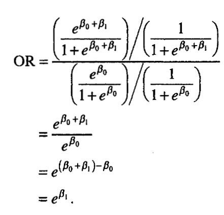
This is why you can exponentiate the co-efficients from logistic regression to derive the odds ratio- note we start out with calculating the odds given X =1 and divide that by the odds given X = 0  for exp( Bo + B1X ). See logistic regression and the calculation and interpretation of odds ratios  and analysis of the logistic function for more details.

Back Propagation

In a recent post on neural networks, using R I described neural networks and presented the following visualization from R:

 I have also described a multilayer perceptron as a weighted average or ensemble of logits. But how are the weights in each hidden layer logistic activation function (or any activation function for other network architectures) estimated? How are the weights in the combination functions estimated? Neural networks can be estimated using back propagation, described in Hastie as 'a generic approach to minimizing R(θ) (the cost function) by gradient descent.'

Given a neural network with inputs X with hidden layers comprised of hidden units Z used to predict some target T,  we can represent a neural network schematically (simplifying the notation in Hastie by omitting key subscripts and summations)

X -> Z -> T

Z = σ( α₀ +  α^Tx)
T =  β₀ + βZ
f(X) = g(T)   [1]

where σ = the activation function

Given weights {α₀,α₀ ,  β₀ , β} find the values that minimize the specified error function:

R(θ) =∑∑ ( y-f(x)² )      [2] (note a number of possible error functions may be used)

Backpropogation equations:

s = σ'( α^Tx )βδ   [3]

Errors can be re-specified as:

∂R/ ∂β = δZ   [4]

∂R/ ∂α = sx    [5]

Gradient Descent Update:

β^r+1 =  β^r - γ ∂R/ ∂β    [6]

α^r+1 =  α^r - γ ∂R/ ∂α   [7]

Algorithm:

Forward Pass: use initial or current weights (guesses) and calculate f(X), and errors δ from the output layer [2]

Backward Pass:  'back propagate' via back propagation equation [3] to obtain s. Both sets of errors (δ) and (s) are used to derive the derivative terms in [4] and [5]  which are then used in the gradient descent update weight estimates via equations [6]& [7].

In Predictive modeling with SAS Enterprise Miner by Sarma,  the following basic description of back propagation is given:

Specify an error function E.

1) 1st iteration- set initial weights, use to evaluate E

2) 2nd iteration- weights are changed by a small amount such that the error is redced

-repeat until convergence

As Sarma explains, with each iteration a number of weights are produced, so if it takes 100 iterations to converge, 100 possible models are specified, giving 100 sets of weights. Using validation data, the best iteration can be chosen calculating E via the validation data.

Gradient Descent

The following lecture from Dr. Ng's course in machine learning from Stanford covers gradient descent.





When I first sat through this lecture I wondered if it would really be useful. It turns out that understanding gradient descent is helpful to understanding backpropogation which is used to train neural networks.

 Based on the lecture notes, gradient descent can be described as follows:

Suppose we want to predict y with a function h(x) =  Θ₀+ Θ₁ x₁ + x₂Θ₂ + etc =  Θ^Tx  or βX

given a specified cost function: J(Θ) = (1/2) ∑  (h(x)-y)²or    e'e

we choose  Θ to minimize J(Θ) using a search algorithm that repeatedly changes Θ to make J(Θ) smaller and smaller until it converges to a value of Θ that minimizes J(Θ).

Θ : Θ(i) - α ∂ J(Θ)/∂Θ(i)  or β : βi - α ∂e'e/∂β  'update or guessing function' for some guess 'i'

Solving for the partial derivative or gradient term gives:

∂ J(Θ)/∂Θ(i) = (h(Θ)-y)x   or e'x

and the update function becomes:

Θ: Θ(i) +α(y-h(x))x   or β : βi - αe'x

the magnitude of each update for each iteration is a function of the error term and the learning rate 'α '.

Alternatively, gradient descent can be represented as follows:

Given a function F() and guess Xo and the update function

Xn+1 = Xn - α∇F(Xn)

we get a series of updates such that F(Xo) > F(X1) > F(X2) >F(X3...

with convergence at the minimum value of F().

Instrumental Variables and Selection Bias

In a previous post I noted Hal Varian and Andrew Gelman's discussion on instrumental variables, and the following specification for program or treatment T and instrument Z :

"You have to assume that the only way that z affects Y is through the treatment, T. So the IV model is
 
T = az + e 1 

y = bT + d    

It follows that

E(y|z) = b E(T|z) + E(d|z)

Now if we
1) assume E(d|z) = 0
2) verify that E(T|z) != 0
 

we can solve for b by division

i.e. b = E(y|z) / E(T|z)

 In a recent paper 'Using Instrumental Variables to Account for Selection Effects in Research on First Year Programs' Pike, Hansen and Lin expand on the details following  the work of Angrist and Pischke. They describe selection bias for participation in first year programs at 4 year universities in the context of omitted variable bias.

 Yi = α + βjXij + pDi + η

where Xij may or may not be related to Di, which is program participation.
          p = the unbiased effect of program participation

and η = γSi +  v

Given that γSi is related to program participation, it causes the effect of program participation to be overstated.

Pike, Hansen and Lin propose capturing the impact of selection bias using instrumental variables  (Z) to ultimately measure the impact of program participation, p.

 p = cov(Y, Z)/ cov(D, Z) = Π11 / Π21

Where impact of program participation is derived from the ratio of two regressions, Y on Z  and D on Z.

 Y = α1 + βX + Π11Z + e1
 D = α2 + βX + Π21Z + e2

As they explain in their paper, the ratio for p as it is defined above is useful in thinking about the consequences of the two major assumptions of IV analysis.

1) Z should be strongly correlated with D. If the correlation is week, then the denominator will  be small, and p will be overstated.

2) Z should be unrelated to Y and 'e'. If the correlation is strong, then the numerator will be large, and p will overstate program effects.

 In the paper, they correct for the impact of selection bias using two instruments (participation in a summer bridge program and having decided a major prior to enrollment). In a normal regression, they find that even after correcting for various other controls, there is a positive significant relationship between first year programs and student success (measured by GPA). However, by including the instruments in the regression (correcting for selection bias) this relationship goes away.

Instrumental variable techniques add a valuable tool that all policy analysts and researchers should have in their quantitative tool box. As stated in the paper:

"If, as the results of this study suggest, traditional evaluation methods can overstate (either positively or negatively) the magnitude of program effects in the face of self selection, then evaluation research may be providing decision makers with inaccurate information. In addition to providing an incomplete accounting for external audiences, inaccurate information about program effectiveness can lead to the misallocation of scarce institutional resources."

References: 

Angrist and Pischke, Mostly Harmless Econometrics, 2009 

Using Instrumental Variables to Account for Selection Effects in Research on First-Year Programs
Gary R. Pike, Michele J. Hansen and Ching-Hui Lin
Research in Higher Education
Volume 52, Number 2, 194-214, DOI: 10.1007/s11162-010-9188-x 

Vector Autoregressions and Bayesian Vector Autoregressions

In a previous post I highlighted the basic algebra associated with ARIMA models:

  

Ex ARMA(2,1,1) : ( Y*_t = b₀ + b₁Y*_t-1  + b₂Y*_t-2  + b₃ e_t-1  + e_t

The terms in this model consist only of a single observed time series and its associated error terms. Vector Autoregressions (VAR's) are class of models that allow for a multivariate analysis of time series. For example 2 series Y₁  and Y₂ (perhaps GNP and treasury yields). We could specify the two series as follows:

Y_1,t  =  c₁ + A_1,1Y_1,t-1 + A_1,2Y_2,t-1 + e_1,t

Y_2,t  =  c₂ + A_2,1Y_1,t-1 + A_2,2Y_2,t-1 + e_2,t    

 

More generally, writing one equation for each series:

Y_t  =  c + A₁Y_t-1 + …+ A_pY_t-p + e

  

Or in matrix form: Y = AZ + U

Y =  series of K different endogenous variables

A=  coefficient matrix

Z =  matrix of lagged variables

U = matrix of error terms

Exogenous variables ‘x’ can be incorporated as follows:

  Y_t  =  c + A₁Y_t-1 + …+ A_pY_t-p + B₁X_t-1 + …+ B_pX_t-p + u

Problems with VAR’s

Given the large number of parameters in VAR’s, overparamaterization and over fitting becomes an issue. Some coefficients may turn out to be different from zero by coincidence, leading to spurious relationships in the model specification.

Bayesian Vector Auto regression (BVAR)

Assume that the model parameters are random variable. A prior distribution is specified based on prior information and combined with objective information from observed data to obtain the posterior distribution using Bayes Theorem.  The prior distribution specification acts as a barrier, or provides ‘shrinkage’ preventing the estimated parameters from depicting what are only spurious correlations.

Estimation

Recall , Bayes Theorem, for parameter θ  and data X,  in its simplest form:

p(θ |X) = p(X|θ)p(θ ) / p(X)  or  p(X|θ)p(θ ) / ∑_i p(X| θ_i) p(θ_i)

The posterior distribution can be defined based on the prior and the likelihood function as follows:

p(θ|X) = p(θ ) L(θ|X) / ∫_θ p(θ) L(θ |X) dθ α p(θ) L(θ |X)

This should look familiar- see also the post on Bayesian Econometrics.

p(θ|X) is then estimated based on the above formulation using MCMC methods. Various prior distributions have been discussed in the literature, including the Minnessota Prior, Conjugate Priors, Flat Priors, and the Sims-Zha Prior.

References:

The Usage of Different Prior Distributions in Bayesian Vector Autoregressive Models. Volkan Sevinc and Gul Ergun. Hacettepe Journal of Mathematics and Statistics Volume 38(1) 2009.

Advances in Bayesian Time Series Modeling and the Study of Politics: Theory, Testing, Forecasting, and Policy Analysis. Patrick T. Brandt and John R. Freeman. Political Analysis. (2006) 14:1-36.

Vector Autoregression. (presentation) Jamie Monogan. Washington University. St. Louis. November 15 & 17, 2010. Link: http://artsci.wustl.edu/~jmonogan/teaching/ts/14var.pdf

Maximum Likelihood Estimation Visualization with SAS and R

 (see also Algorithms for Maximum Likelihood Estimation)

I recently found some notes posted for a biostatistics course at the University of Minnesota, (I believe it was taught by John Connet) which presented SAS code for implementing  maximum likelihood estimation using Newton's method via PROC IML.  As noted in my post on logistic regression:

When we undertake MLE we typically maximize the log of the likelihood function as follows:

Max Log(L(β)) or LL ‘log likelihood’ or solve:

∂Log(L(β))/∂β = 0  

As noted in the biostats course notes, typically we can't solve for these formulas directly, but the solutions have to be estimated iteratively. One method of doing this is Netwon's Method, which the IML code implements. (see SAS code that follows below)

After simulating the data and running the procedure, the algorithm converges in  6 steps, (i.e. the solutions for the  β estimates are reached in 6steps). Below is summary of the results:

Also, plotting these via PROC G3D, (with my crude annotations) shows how with each step or iteration of the algoritm, we get closer and closer to maximiizing the log of the likelihood function.



Note, running PROC LOGISTIC  (which actually implements Fisher Scoring) against the simulated data gives very similar results to the algorithm implemented in PROC IML:

Note, given certain assumptions, you can get similar results from implementing least squares and maximum likelihood. If we make the following assumptions:

And we specify a likelihood function based on the normal density:

Maximizing this with respect to the β 's  will give the same least squares results.

Using R (code below) I simulated data and specified the likelihood function above for a single variable regression.  (for more info see Ajay Shah's notes , as well as Maximum Likelihood Programming in R)

Running a regression on the simulated data  (using R's 'lm' operation) produced the following results:

Coefficients:

            Estimate Std. Error t value Pr(>|t|)   
(Intercept)   1.9910     0.1961  10.156  < 2e-16 ***
X[, 2]        2.9102     0.3418   8.514 2.01e-13 ***
---
Signif. codes:  0 ‘***’ 0.001 ‘**’ 0.01 ‘*’ 0.05 ‘.’ 0.1 ‘ ’ 1

Residual standard error: 0.9693 on 98 degrees of freedom

Multiple R-squared: 0.4252,     Adjusted R-squared: 0.4193
F-statistic: 72.48 on 1 and 98 DF,  p-value: 2.009e-13

The 'beta' coefficeint on x is 2.9102 . Using the R function 'optim' I optimized the likelihood function, getting the results below, which are on par with the actual regression I just ran above:

$par

[1] 1.9910299 2.9101836 0.9207324

In order B0 =  1.9910299  and B1 = 2.9101836  which are the results we got before.

Iterating values for B1 and using the R 'apply' function in conjunction with the specified likelihood function, I plotted the values of the likelihood function for each iterated value of B1. As shown, the likelihood function is maximized at B1 ~ 2.9101836

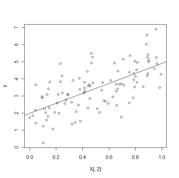
And below is the OLS line (with the same beta's we get from maximum likelihood above) plotted against the simulated data:

SAS Code Below:

/* PROC IML MLE SIMULATION */

/*    Program to compute maximum likelihood estimates ....           */;

/*    Based on Newton-Raphson methods - uses IML                     */;

footnote "program: /home/walleye/john-c/5421/imlml.sas &sysdate &systime" ;

options linesize = 80 ;

data sim ;

     one = 1 ;

     a = 2 ;

     b = 1 ;

     n = 300 ;

     seed = 20000214 ;

/*   Simulated data from logistic distribution                      */;

     do i = 1 to n ;

        u = 2 * i / n ;

        p = 1 / (1 + exp(-a - b * u)) ;

        r = ranuni(seed) ;

        yi = 0 ;

        if r lt p then yi = 1 ;

        output ;

     end ;

run ;

/*look at data */

proc univariate data = sim;

var p;

histogram p;

run;

/*   Logistic analysis of simulated data ......                     */;

proc logistic descending data = sim outmodel = logit;

     model yi = u / lackfit rsq;

        score data =sim out= score1 fitstat ;

title1 'Proc logistic results ... ' ;

run ;

/*   Begin proc iml ..............................                    */;

title1 'PROC IML Results ...' ;

proc iml ;

  use sim ;                        /* Input the simulated dataset     */;

  read all var {one u} into x ;    /* Read the design matrix into x   */;

  read all var {yi}    into y ;    /* Read the outcome data into y    */;

  p = 2 ;                          /* Set the number of parameters    */;

  beta = {0.00, 0.00} ;            /* Initialize the param. vector    */;

/* -------------------------------------------------------------------*/;

/*   Module which computes loglikelihood and derivatives ...          */;

  start loglike(beta, p, x, y, l, dl, d2l) ;

     n = 300 ;

     l = 0 ;                       /*  Initialize log likelihood ...  */;

     dl  = j(p, 1, 0) ;            /*  Initialize 1st derivatives...  */;

     d2l = j(p, p, 0) ;            /*  Initialize 2nd derivatives...  */;

     do i = 1 to n ;

        xi = x[i,] ; 

        yi = y[i] ;

        xibeta = xi * beta ;

        w = exp(-xibeta) ;

/*      The log likelihood for the i-th observation ...               */;

        iloglike = log((1 - yi) * w + yi) - log(1 + w) ;

        l = l + iloglike ;

        do j = 1 to p ;

           xij = xi[j] ;

/*      The jth 1st derivative of the log likelihood for the ith obs      */;

           jdlogl = -(1 - yi) * w * xij / ((1 - yi) * w + yi)

                    + w * xij / (1 + w) ;

           dtemp = dl[j] + jdlogl ;

           dl[j] = dtemp ;

           do k = 1 to p ;

              xik = xi[k] ;

/*      The jkth 2nd derivative of the log likelihood for the ith obs    */;

              jkd2logl = ((1 - yi) * w * xij * xik * ((1 - yi) * w + yi)

                         -(1 - yi) * w * xij * ((1 - yi) * w * xik))/

                          ((1 - yi) * w + yi)**2

                       + (-w * xij * xik * (1 + w) + w * w * xij * xik)/

                          (1 + w)**2 ;

              d2temp = d2l[j, k] ;

              d2l[j, k] = d2temp + jkd2logl ;

           end ;

        end ;

     end ;

 finish loglike ;

/* -------------------------------------------------------------------*/;

 eps = 1e-8 ;

 diff = 1 ;

/*  The following do loop stops when the increments in beta are       */;

/*  sufficiently small, or when number of iterations reaches 20       */;

 do iter = 1 to 20 while(diff > eps) ;

    run loglike(beta, p, x, y, l, dl, d2l) ;

    invd2l = inv(d2l) ;

    beta = beta - invd2l * dl ;       /*  The key Newton step ...  */;

    diff = max(abs(invd2l * dl)) ;

    print iter  l  dl  d2l  diff  beta ;

 end ;

 b1 = beta[1] ;

 b2 = beta[2] ;

 serr1 = sqrt(-invd2l[1, 1]) ;

 serr2 = sqrt(-invd2l[2, 2]) ;

 covar = -invd2l ;

 llratio = - 2 * l ;

 print ' -2 * loglikelihood = ' llratio ;

 print 'b1 coeff, std err : ' b1 serr1 ;

 print 'b2 coeff, std err : ' b2 serr2 ;

 print 'covariance matrix : ' covar ;

quit ;

/* read the values of LL and beta's into a SAS data set*/

data ldat;

input B1 B2 LL;

cards;

1.424660 0.2810698 -207.90000

1.689885 0.6639477  -86.11339

1.628445 1.0044749  -76.10077

1.593570 1.1053311  -74.93779

1.591699 1.1108087  -74.89053

1.591694 1.1108238  -74.89040

;

run;

PROC G3D DATA=ldat GOUT=THECAT;

  

   SCAT B1 * B2 = LL / GRID  SIZE=1  COLOR='GREEN' XTICKNUM =10 YTICKNUM =10;

TITLE'';

   RUN; QUIT;

R Code Below:

# *------------------------------------------------------------------
# | PROGRAM NAME: mle_sim
# | DATE: 5/15/11
# | CREATED BY:  Matt Bogard
# | PROJECT FILE:  econometric sense            
# *----------------------------------------------------------------
# | PURPOSE: demonstrate mle in R              
# |
# *------------------------------------------------------------------
# | COMMENTS:               
# |
# |  1: see also: Maximum Likelihood Programming in R Marco R. Steenbergen 
# |       http://www.artsci.wustl.edu/~jmonogan/computing/r/MLE_in_R.pdf
# |  2: notes from: Ajay Sha -'Roll Your Own Likelihood Function in R here: http://www.mayin.org/ajayshah/KB/R/documents/mle/mle.html 
# |  3: Ajay also has lots of other R by example links here: http://www.mayin.org/ajayshah/KB/R/
# |*------------------------------------------------------------------
#
 
 
# simulate data for x
set.seed(123)
 
X<-cbind(1,runif(100))
dim(X)
 
 
# set true values for the betas and variance
 
theta.true<-c(2,3,1) # B0, B1, sigma^2
 
# generate  y-values
 
y<-X%*%theta.true[1:2] + rnorm(100)
dim(y)
 
plot(y~X[,2])
 
 
# specify the likelihood function based on the standard normal distribution
 
ols.lf<-function(theta,y,X){ n<-nrow(X)
k<-ncol(X)
beta<-theta[1:k]
sigma2<-theta[k+1]
e<-y-X%*%beta
logl<- -.5*n*log(2*pi)-.5*n*log(sigma2)-
((t(e)%*%e)/(2*sigma2))
return(-logl)
}
 
 
# optimize the likelihood function with initial values for BO, B1, sigma^2 -> 1,1,1
 
p<-optim(c(1,1,1),ols.lf,method="BFGS",hessian=T,y=y,X=X)
 
names(p)
 
print(p)
 
 
# note SE(B) =  square root of the diagonals of the inverse of the hession
 
OI<-solve(p$hessian)
 
se<-sqrt(diag(OI))
 
 
# compare to linear model
 
d<-summary(lm(y~X[,2]))
 
 
# plotting 
 
theta.ols <- c(sigma2 = d$sigma^2, d$coefficients[,1])  # get linear model betas from output
theta <- theta.ols  # theta for next simulation
delta.values <- seq(-1.5, 1.5, .01)  # iterate beta values by amounts between -1.5 and 1.5
 
logl.values <- as.numeric(lapply(delta.values,
                                 function(x) {-ols.lf(theta+c(0,0,x),y,X)}))  # this produces log likelihood values for values of X,y,and iterated beta's
 
#  plot likelihood function and betas 
plot(theta[3]+delta.values, logl.values, type="l", lwd=3, col="blue",
     xlab="B1", ylab="Log likelihood")

Created by Pretty R at inside-R.org