Maximum Likelihood Estimation Visualization with SAS and R

 (see also Algorithms for Maximum Likelihood Estimation)

I recently found some notes posted for a biostatistics course at the University of Minnesota, (I believe it was taught by John Connet) which presented SAS code for implementing  maximum likelihood estimation using Newton's method via PROC IML.  As noted in my post on logistic regression:

When we undertake MLE we typically maximize the log of the likelihood function as follows:

Max Log(L(β)) or LL ‘log likelihood’ or solve:

∂Log(L(β))/∂β = 0  

As noted in the biostats course notes, typically we can't solve for these formulas directly, but the solutions have to be estimated iteratively. One method of doing this is Netwon's Method, which the IML code implements. (see SAS code that follows below)

After simulating the data and running the procedure, the algorithm converges in  6 steps, (i.e. the solutions for the  β estimates are reached in 6steps). Below is summary of the results:

Also, plotting these via PROC G3D, (with my crude annotations) shows how with each step or iteration of the algoritm, we get closer and closer to maximiizing the log of the likelihood function.



Note, running PROC LOGISTIC  (which actually implements Fisher Scoring) against the simulated data gives very similar results to the algorithm implemented in PROC IML:

Note, given certain assumptions, you can get similar results from implementing least squares and maximum likelihood. If we make the following assumptions:

And we specify a likelihood function based on the normal density:

Maximizing this with respect to the β 's  will give the same least squares results.

Using R (code below) I simulated data and specified the likelihood function above for a single variable regression.  (for more info see Ajay Shah's notes , as well as Maximum Likelihood Programming in R)

Running a regression on the simulated data  (using R's 'lm' operation) produced the following results:

Coefficients:

            Estimate Std. Error t value Pr(>|t|)   
(Intercept)   1.9910     0.1961  10.156  < 2e-16 ***
X[, 2]        2.9102     0.3418   8.514 2.01e-13 ***
---
Signif. codes:  0 ‘***’ 0.001 ‘**’ 0.01 ‘*’ 0.05 ‘.’ 0.1 ‘ ’ 1

Residual standard error: 0.9693 on 98 degrees of freedom

Multiple R-squared: 0.4252,     Adjusted R-squared: 0.4193
F-statistic: 72.48 on 1 and 98 DF,  p-value: 2.009e-13

The 'beta' coefficeint on x is 2.9102 . Using the R function 'optim' I optimized the likelihood function, getting the results below, which are on par with the actual regression I just ran above:

$par

[1] 1.9910299 2.9101836 0.9207324

In order B0 =  1.9910299  and B1 = 2.9101836  which are the results we got before.

Iterating values for B1 and using the R 'apply' function in conjunction with the specified likelihood function, I plotted the values of the likelihood function for each iterated value of B1. As shown, the likelihood function is maximized at B1 ~ 2.9101836

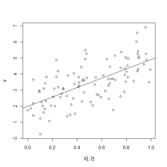
And below is the OLS line (with the same beta's we get from maximum likelihood above) plotted against the simulated data:

SAS Code Below:

/* PROC IML MLE SIMULATION */

/*    Program to compute maximum likelihood estimates ....           */;

/*    Based on Newton-Raphson methods - uses IML                     */;

footnote "program: /home/walleye/john-c/5421/imlml.sas &sysdate &systime" ;

options linesize = 80 ;

data sim ;

     one = 1 ;

     a = 2 ;

     b = 1 ;

     n = 300 ;

     seed = 20000214 ;

/*   Simulated data from logistic distribution                      */;

     do i = 1 to n ;

        u = 2 * i / n ;

        p = 1 / (1 + exp(-a - b * u)) ;

        r = ranuni(seed) ;

        yi = 0 ;

        if r lt p then yi = 1 ;

        output ;

     end ;

run ;

/*look at data */

proc univariate data = sim;

var p;

histogram p;

run;

/*   Logistic analysis of simulated data ......                     */;

proc logistic descending data = sim outmodel = logit;

     model yi = u / lackfit rsq;

        score data =sim out= score1 fitstat ;

title1 'Proc logistic results ... ' ;

run ;

/*   Begin proc iml ..............................                    */;

title1 'PROC IML Results ...' ;

proc iml ;

  use sim ;                        /* Input the simulated dataset     */;

  read all var {one u} into x ;    /* Read the design matrix into x   */;

  read all var {yi}    into y ;    /* Read the outcome data into y    */;

  p = 2 ;                          /* Set the number of parameters    */;

  beta = {0.00, 0.00} ;            /* Initialize the param. vector    */;

/* -------------------------------------------------------------------*/;

/*   Module which computes loglikelihood and derivatives ...          */;

  start loglike(beta, p, x, y, l, dl, d2l) ;

     n = 300 ;

     l = 0 ;                       /*  Initialize log likelihood ...  */;

     dl  = j(p, 1, 0) ;            /*  Initialize 1st derivatives...  */;

     d2l = j(p, p, 0) ;            /*  Initialize 2nd derivatives...  */;

     do i = 1 to n ;

        xi = x[i,] ; 

        yi = y[i] ;

        xibeta = xi * beta ;

        w = exp(-xibeta) ;

/*      The log likelihood for the i-th observation ...               */;

        iloglike = log((1 - yi) * w + yi) - log(1 + w) ;

        l = l + iloglike ;

        do j = 1 to p ;

           xij = xi[j] ;

/*      The jth 1st derivative of the log likelihood for the ith obs      */;

           jdlogl = -(1 - yi) * w * xij / ((1 - yi) * w + yi)

                    + w * xij / (1 + w) ;

           dtemp = dl[j] + jdlogl ;

           dl[j] = dtemp ;

           do k = 1 to p ;

              xik = xi[k] ;

/*      The jkth 2nd derivative of the log likelihood for the ith obs    */;

              jkd2logl = ((1 - yi) * w * xij * xik * ((1 - yi) * w + yi)

                         -(1 - yi) * w * xij * ((1 - yi) * w * xik))/

                          ((1 - yi) * w + yi)**2

                       + (-w * xij * xik * (1 + w) + w * w * xij * xik)/

                          (1 + w)**2 ;

              d2temp = d2l[j, k] ;

              d2l[j, k] = d2temp + jkd2logl ;

           end ;

        end ;

     end ;

 finish loglike ;

/* -------------------------------------------------------------------*/;

 eps = 1e-8 ;

 diff = 1 ;

/*  The following do loop stops when the increments in beta are       */;

/*  sufficiently small, or when number of iterations reaches 20       */;

 do iter = 1 to 20 while(diff > eps) ;

    run loglike(beta, p, x, y, l, dl, d2l) ;

    invd2l = inv(d2l) ;

    beta = beta - invd2l * dl ;       /*  The key Newton step ...  */;

    diff = max(abs(invd2l * dl)) ;

    print iter  l  dl  d2l  diff  beta ;

 end ;

 b1 = beta[1] ;

 b2 = beta[2] ;

 serr1 = sqrt(-invd2l[1, 1]) ;

 serr2 = sqrt(-invd2l[2, 2]) ;

 covar = -invd2l ;

 llratio = - 2 * l ;

 print ' -2 * loglikelihood = ' llratio ;

 print 'b1 coeff, std err : ' b1 serr1 ;

 print 'b2 coeff, std err : ' b2 serr2 ;

 print 'covariance matrix : ' covar ;

quit ;

/* read the values of LL and beta's into a SAS data set*/

data ldat;

input B1 B2 LL;

cards;

1.424660 0.2810698 -207.90000

1.689885 0.6639477  -86.11339

1.628445 1.0044749  -76.10077

1.593570 1.1053311  -74.93779

1.591699 1.1108087  -74.89053

1.591694 1.1108238  -74.89040

;

run;

PROC G3D DATA=ldat GOUT=THECAT;

  

   SCAT B1 * B2 = LL / GRID  SIZE=1  COLOR='GREEN' XTICKNUM =10 YTICKNUM =10;

TITLE'';

   RUN; QUIT;

R Code Below:

# *------------------------------------------------------------------
# | PROGRAM NAME: mle_sim
# | DATE: 5/15/11
# | CREATED BY:  Matt Bogard
# | PROJECT FILE:  econometric sense            
# *----------------------------------------------------------------
# | PURPOSE: demonstrate mle in R              
# |
# *------------------------------------------------------------------
# | COMMENTS:               
# |
# |  1: see also: Maximum Likelihood Programming in R Marco R. Steenbergen 
# |       http://www.artsci.wustl.edu/~jmonogan/computing/r/MLE_in_R.pdf
# |  2: notes from: Ajay Sha -'Roll Your Own Likelihood Function in R here: http://www.mayin.org/ajayshah/KB/R/documents/mle/mle.html 
# |  3: Ajay also has lots of other R by example links here: http://www.mayin.org/ajayshah/KB/R/
# |*------------------------------------------------------------------
#
 
 
# simulate data for x
set.seed(123)
 
X<-cbind(1,runif(100))
dim(X)
 
 
# set true values for the betas and variance
 
theta.true<-c(2,3,1) # B0, B1, sigma^2
 
# generate  y-values
 
y<-X%*%theta.true[1:2] + rnorm(100)
dim(y)
 
plot(y~X[,2])
 
 
# specify the likelihood function based on the standard normal distribution
 
ols.lf<-function(theta,y,X){ n<-nrow(X)
k<-ncol(X)
beta<-theta[1:k]
sigma2<-theta[k+1]
e<-y-X%*%beta
logl<- -.5*n*log(2*pi)-.5*n*log(sigma2)-
((t(e)%*%e)/(2*sigma2))
return(-logl)
}
 
 
# optimize the likelihood function with initial values for BO, B1, sigma^2 -> 1,1,1
 
p<-optim(c(1,1,1),ols.lf,method="BFGS",hessian=T,y=y,X=X)
 
names(p)
 
print(p)
 
 
# note SE(B) =  square root of the diagonals of the inverse of the hession
 
OI<-solve(p$hessian)
 
se<-sqrt(diag(OI))
 
 
# compare to linear model
 
d<-summary(lm(y~X[,2]))
 
 
# plotting 
 
theta.ols <- c(sigma2 = d$sigma^2, d$coefficients[,1])  # get linear model betas from output
theta <- theta.ols  # theta for next simulation
delta.values <- seq(-1.5, 1.5, .01)  # iterate beta values by amounts between -1.5 and 1.5
 
logl.values <- as.numeric(lapply(delta.values,
                                 function(x) {-ols.lf(theta+c(0,0,x),y,X)}))  # this produces log likelihood values for values of X,y,and iterated beta's
 
#  plot likelihood function and betas 
plot(theta[3]+delta.values, logl.values, type="l", lwd=3, col="blue",
     xlab="B1", ylab="Log likelihood")

Created by Pretty R at inside-R.org