Back in 2012 I wrote about the basic 2 x 2 difference in difference analysis (two groups, two time periods). Columbia public health probably has a better introduction.
The most famous example of an analysis that motivates a 2 x 2 DID analysis is John Snow's 1855 analysis of the cholera epidemic in London:
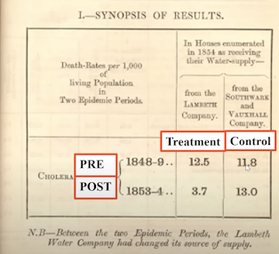
(Image Source)
I have since written about some of the challenges of estimating DID with glm models (see here, here, and here.), as well as combining DID with matching, and problems to watch out for when combining methods. But a lot of what we know about difference in differences has changed in the last decade. I'll try to give a brief summary based on my understanding and point towards some references that do a better job presenting the current state.
The Two-Way Fixed Effects model (TWFE)
The first thing I should discuss is extending the 2x2 model to include multiple treated groups and/or multiple time periods. The generalized model for DiD also referred to as the two-way fixed effects (TWFE) model is the best way to represent those kind of scenarios:.
Ygt = ag + bt + δDgt + εt
ag = group fixed effects
bt = time fixed effects
Dgt= treatment*post period (interaction term)
δ = ATT or DID estimate
Getting the correct standard errors for DID models that involve many repeated measures over time and/or where treatment and control groups are defined by multiple geographies presents two challenges compared to the basic 2x2 model. Serial correlation and correlation within groups. There are several approaches that can be considered depending on your situation.
1 - Block bootstrapping
2 - Aggregating data into single pre and post periods
3 - Clustering standard errors at the group level
Clustering at the group level should provide the appropriate standard errors in these situations when the number of clusters are large.
For more details on TWFE models, both Scott Cunningham and Nick Huntington-Klein have great econometrics textbooks with chapters devoted to these topics. See the references below for more info.
Differential Timing and Staggered Rollouts
But things can get even more complicated with DID designs. Think about situations where there are different groups getting treated at different times over a number of time periods. This is not just a thought experiment trying to imagine the most difficult study design and pondering for the sake of pondering – these kind of staggered rollouts are very common in business and policy settings. Imagine policy rules adopted by different states over time (like changes in minimum wages) or imagine testing a new product or service by rolling it out to different markets over time. Understanding how to evaluate their impact is important. For a while it seemed economists may have been a little guilty of handwaving with the TWFE model assuming the estimated treatment coefficient was giving them the effect they wanted.
But Andrew Goodman-Bacon refused to take this interpretation at face value and broke this down for us determining that the TWFE estimator was trying to give us a weighted average of all potential 2x2 DID estimates you could make with the data. That actually sounds intuitive and helpful. But what he discovered that is not so intuitive is that some of those 2x2 comparisons could be comparing previously treated groups with current treated groups. That's not a comparison we generally are interested in making, but it gets averaged in with the others and can drastically bias the results particularly when there is treatment effect heterogeneity (the treatment effect is different across groups and trending over time).
So how do you get a better DID estimate in this situation? I'll spare you the details (because I'm still wrestling with them) but the answer seems to be the estimation strategy developed by Callaway and Sant'Anna. The documentation in R for their package walks through a lot of the details and challenges with TWFE models with differential timing.
Additionally this video of Andrew Goodman-Bacon was really helpful for understanding the 'Bacon' decomposition of TWFE models and the problems above.
After watching Goodman-Bacon, I recommend this talk from Sant'Anna discussing their estimator.
Below Nick Huntington-Klein provides a great summary of the issues made apparent by the Bacon decomposition made above and the Callaway and Sant'Anna method for staggered/rollout DID designs. he also gets into the Wooldridge Mundlack approach:
A Note About Event Studies
In a number of references I have tried to read to understand this issue, the term 'event study' is thrown around and it seems like every time it is used it is used differently but the author/speaker assumes we are all taking about the same thing. In this video Nick Huntington-Klein introduces event studies in a way that is the most clear and consistent. Watching this video might help.
References:
Causal Inference: The Mixtape. Scott Cunningham. https://mixtape.scunning.com/
The Effect: Nick Huntington-Klein. https://theeffectbook.net/
Andrew Goodman-Bacon. Difference-in-differences with variation in treatment timing. Journal of Econometrics.Volume 225, Issue 2, 2021.
Brantly Callaway, Pedro H.C. Sant’Anna. Difference-in-Differences with multiple time periods. Journal of Econometrics. Volume 225, Issue 2, 2021,
Related Posts:
Modeling Claims Costs with Difference in Differences. https://econometricsense.blogspot.com/2019/01/modeling-claims-with-linear-vs-non.html
Was It Meant to Be? OR Sometimes Playing Match Maker Can Be a Bad Idea: Matching with Difference-in-Differences. https://econometricsense.blogspot.com/2019/02/was-it-meant-to-be-or-sometimes-playing.html