I actually have not created a post related generalized method of moments. Until then, this video seems to provide a nice introduction if you are already comfortable with he concept of moments and method of moments estimation.
As noted, the full video and slides can also be found here:
Showing posts with label optimization. Show all posts
Showing posts with label optimization. Show all posts
Wednesday, September 5, 2012

Sunday, November 27, 2011
Regression via Gradient Descent in R
In a previous post I derived the least squares estimators using basic calculus, algebra, and arithmetic, and also showed how the same results can be achieved using the canned functions in SAS and R or via the matrix programming capabilities offered by those languages. I've also introduced the concept of gradient descent here and here.
Given recent course work in the online machine learning course via Stanford, in this post, I tie all of the concepts together. The R -code that follows borrows heavily from the Statalgo blog, which has done a tremendous job breaking down the concepts from the course and applying them in R. This is highly redundant to that post, but not quite as sophisticated (i.e. my code isn't nearly as efficient), but it allows me to intuitively extend the previous work I've done.
If you are not going to use a canned routine from R or SAS to estimate a regression, then why not at least apply the matrix inversions and solve for the beta's as I did before? One reason may be that with a large number of features (independent variables) the matrix inversion can be slow, and a computational algorithm like gradient descent may be more efficient.
From my earliest gradient descent post, I provided the intuition and notation necessary for performing gradient descent to estimate OLS coefficients. Following the notation from the machine learning course mentioned above, I review the notation again below.
In machine learning, the regression function y = b0 + b1x is referred to as a 'hypothesis' function:


(see here for a basic demo using R code)


Created by Pretty R at inside-R.org
Given recent course work in the online machine learning course via Stanford, in this post, I tie all of the concepts together. The R -code that follows borrows heavily from the Statalgo blog, which has done a tremendous job breaking down the concepts from the course and applying them in R. This is highly redundant to that post, but not quite as sophisticated (i.e. my code isn't nearly as efficient), but it allows me to intuitively extend the previous work I've done.
If you are not going to use a canned routine from R or SAS to estimate a regression, then why not at least apply the matrix inversions and solve for the beta's as I did before? One reason may be that with a large number of features (independent variables) the matrix inversion can be slow, and a computational algorithm like gradient descent may be more efficient.
From my earliest gradient descent post, I provided the intuition and notation necessary for performing gradient descent to estimate OLS coefficients. Following the notation from the machine learning course mentioned above, I review the notation again below.
In machine learning, the regression function y = b0 + b1x is referred to as a 'hypothesis' function:
The idea, just like in OLS is to minimize the sum of squared errors, represented as a 'cost function' in the machine learning context:

This is minimized by solving for the values of theta that set the derivative to zero. In some cases this can be done analytically with calculus and a little algebra, but this can also be done (especially when complex functions are involved) via gradient descent. Recall from before, the basic gradient descent algorithm involves a learning rate 'alpha' and an update function that utilizes the 1st derivitive or gradient f'(.). The basic algorithm is as follows:
repeat until convergence {
x := x - α∇F(x)
}
x := x - α∇F(x)
}
(see here for a basic demo using R code)
For the case of OLS, and the cost function J(theta) depicted above, the gradient descent algorithm can be implemented in pseudo-code as follows:
It turns out that:

and the gradient descent algorithm becomes:

The following R -Code implements this algorithm and achieves the same results we got from the matrix programming or the canned R or SAS routines before. The concept of 'feature scaling' is introduced, which is a method of standardizing the independent variables or features. This improves the convergence speed of the algorithm. Additional code intuitively investigates the concept of convergence. Ideally, the algorithm should stop once changes in the cost function become small as we update the values in theta.

The following R -Code implements this algorithm and achieves the same results we got from the matrix programming or the canned R or SAS routines before. The concept of 'feature scaling' is introduced, which is a method of standardizing the independent variables or features. This improves the convergence speed of the algorithm. Additional code intuitively investigates the concept of convergence. Ideally, the algorithm should stop once changes in the cost function become small as we update the values in theta.
R-Code:
#  ----------------------------------------------------------------------------------
# |PROGRAM NAME: gradient_descent_OLS_R
# |DATE: 11/27/11
# |CREATED BY: MATT BOGARD
# |PROJECT FILE:
# |----------------------------------------------------------------------------------
# | PURPOSE: illustration of gradient descent algorithm applied to OLS
# | REFERENCE: adapted from : http://www.cs.colostate.edu/~anderson/cs545/Lectures/week6day2/week6day2.pdf
# |  and http://www.statalgo.com/2011/10/17/stanford-ml-1-2-gradient-descent/
#  ---------------------------------------------------------------------------------

# get data
rm(list = ls(all = TRUE)) # make sure previous work is clear
ls()
x0 <- c(1,1,1,1,1) # column of 1's
x1 <- c(1,2,3,4,5) # original x-values

# create the x- matrix of explanatory variables

x <- as.matrix(cbind(x0,x1))

# create the y-matrix of dependent variables

y <- as.matrix(c(3,7,5,11,14))
m <- nrow(y)

# implement feature scaling
x.scaled <- x
x.scaled[,2] <- (x[,2] - mean(x[,2]))/sd(x[,2])

# analytical results with matrix algebra
 solve(t(x)%*%x)%*%t(x)%*%y # w/o feature scaling
 solve(t(x.scaled)%*%x.scaled)%*%t(x.scaled)%*%y # w/ feature scaling

# results using canned lm function match results above
summary(lm(y ~ x[, 2])) # w/o feature scaling
summary(lm(y ~ x.scaled[, 2])) # w/feature scaling

# define the gradient function dJ/dtheata: 1/m * (h(x)-y))*x where h(x) = x*theta
# in matrix form this is as follows:
grad <- function(x, y, theta) {
  gradient <- (1/m)* (t(x) %*% ((x %*% t(theta)) - y))
  return(t(gradient))
}

# define gradient descent update algorithm
grad.descent <- function(x, maxit){
    theta <- matrix(c(0, 0), nrow=1) # Initialize the parameters

    alpha = .05 # set learning rate
    for (i in 1:maxit) {
      theta <- theta - alpha  * grad(x, y, theta)
    }
 return(theta)
}


# results without feature scaling
print(grad.descent(x,1000))

# results with feature scaling
print(grad.descent(x.scaled,1000))

# -----------------------------------------------------------------------
# cost and convergence intuition
# -----------------------------------------------------------------------

# typically we would iterate the algorithm above until the
# change in the cost function (as a result of the updated b0 and b1 values)
# was extremely small value 'c'. C would be referred to as the set 'convergence'
# criteria. If C is not met after a given # of iterations, you can increase the
# iterations or change the learning rate 'alpha' to speed up convergence

# get results from gradient descent
beta <- grad.descent(x,1000)

# define the 'hypothesis function'
h <- function(xi,b0,b1) {
 b0 + b1 * xi
}

# define the cost function
cost <- t(mat.or.vec(1,m))
  for(i in 1:m) {
    cost[i,1] <-  (1 /(2*m)) * (h(x[i,2],beta[1,1],beta[1,2])- y[i,])^2
  }

totalCost <- colSums(cost)
print(totalCost)

# save this as Cost1000
cost1000 <- totalCost

# change iterations to 1001 and compute cost1001
beta <- (grad.descent(x,1001))
cost <- t(mat.or.vec(1,m))
  for(i in 1:m) {
    cost[i,1] <-  (1 /(2*m)) * (h(x[i,2],beta[1,1],beta[1,2])- y[i,])^2
  }
cost1001 <- colSums(cost)

# does this difference meet your convergence criteria?
print(cost1000 - cost1001)
Gradient Descent in R
In a previous post I discussed the concept of gradient descent. Given some recent work in the online machine learning course offered at Stanford, I'm going to extend that discussion with an actual example using R-code (the actual code is adapted from a computer science course at Colorado State, and the example is verbatim from the notes here: http://www.cs.colostate.edu/~anderson/cs545/Lectures/week6day2/week6day2.pdf )
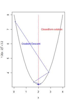
Suppose you want to minimize the function 1.2 * (x-2)^2 + 3.2. Basic calculus requires that we find the 1st derivative and solve for the value of x such that f'(x) = 0. This is easy enough to do, f'(x) = 2*1.2*(x-2). Its easy to see that a value of 2 satisfies f'(x) = 0. Given that the second order conditions hold, this is a minimum.
Its not alwasys the case that we would get a function so easy to work with, and in many cases we may need to numerically estimate the value that minimizes the function. Gradient descent offers a way to do this. Recall from my previous post the gradient descent algorithm can be summarized as follows:
repeat until convergence {
Xn+1 = Xn - α∇F(Xn) or x := x - α∇F(x) (depending on your notational preferences)
}
Where ∇F(x) would be the derivative we calculated above for the function at hand and α is the learning rate. This can easily be implemented R. The following code finds the values of x that minimize the function above and plots the progress of the algorithm with each iteration. (as depicted in the image below)
R-code:
Created by Pretty R at inside-R.org
Suppose you want to minimize the function 1.2 * (x-2)^2 + 3.2. Basic calculus requires that we find the 1st derivative and solve for the value of x such that f'(x) = 0. This is easy enough to do, f'(x) = 2*1.2*(x-2). Its easy to see that a value of 2 satisfies f'(x) = 0. Given that the second order conditions hold, this is a minimum.
Its not alwasys the case that we would get a function so easy to work with, and in many cases we may need to numerically estimate the value that minimizes the function. Gradient descent offers a way to do this. Recall from my previous post the gradient descent algorithm can be summarized as follows:
repeat until convergence {
Xn+1 = Xn - α∇F(Xn) or x := x - α∇F(x) (depending on your notational preferences)
}
Where ∇F(x) would be the derivative we calculated above for the function at hand and α is the learning rate. This can easily be implemented R. The following code finds the values of x that minimize the function above and plots the progress of the algorithm with each iteration. (as depicted in the image below)
R-code:
#  ----------------------------------------------------------------------------------
# |PROGRAM NAME: gradient_descent_R
# |DATE: 11/27/11
# |CREATED BY: MATT BOGARD
# |PROJECT FILE:
# |----------------------------------------------------------------------------------
# | PURPOSE: illustration of gradient descent algorithm
# | REFERENCE: adapted from : http://www.cs.colostate.edu/~anderson/cs545/Lectures/week6day2/week6day2.pdf
# |
#  ---------------------------------------------------------------------------------

xs <- seq(0,4,len=20) # create some values

# define the function we want to optimize

f <-  function(x) {
1.2 * (x-2)^2 + 3.2
}

# plot the function
plot(xs , f (xs), type="l",xlab="x",ylab=expression(1.2(x-2)^2 +3.2))

# calculate the gradeint df/dx

grad <- function(x){
  1.2*2*(x-2)
}


# df/dx = 2.4(x-2), if x = 2 then 2.4(2-2) = 0
# The actual solution we will approximate with gradeint descent
# is  x = 2 as depicted in the plot below

lines (c (2,2), c (3,8), col="red",lty=2)
text (2.1,7, "Closedform solution",col="red",pos=4)


# gradient descent implementation
x <- 0.1 # initialize the first guess for x-value
xtrace <- x # store x -values for graphing purposes (initial)
ftrace <- f(x) # store y-values (function evaluated at x) for graphing purposes (initial)
stepFactor <- 0.6 # learning rate 'alpha'
for (step in 1:100) {
x <- x - stepFactor*grad(x) # gradient descent update
xtrace <- c(xtrace,x) # update for graph
ftrace <- c(ftrace,f(x)) # update for graph
}

lines ( xtrace , ftrace , type="b",col="blue")
text (0.5,6, "Gradient Descent",col="blue",pos= 4)

# print final value of x
print(x) # x converges to 2.0
Wednesday, July 27, 2011
Newton's Method
"Newton's method, also called the Newton-Raphson method, is a root-finding algorithm that uses the first few terms of the Taylor series of a function f(x) in the vicinity of a suspected root." - http://mathworld.wolfram.com/NewtonsMethod.html
Given we want to find some root value x* that optimizes the function f(x) such that f(x*)=0, we start with an initial guess xn and expand around that point with a taylor series:
f(xn + Δx ) = f(xn) + f’(xn)Δx + …=0 where Δx represents the difference between the actual solution x* and the guess xn.
Retaining only the first order terms we can solve for Δx :
Δx = -[f(xn)/f’(xn)]
If xn is an initial guess, the next guess can be obtained by:
xn+1 = xn - [f(xn)/f’(xn)]
Note as we get closer to the true root value x*, f(xn) gets smaller and Δx gets smaller, such that the value xn+1 from the next iteration changes little from the previous. This is referred to as convergence to the root value x*, which optimizes f(x).
Numerical Estimation of Maximum Likelihood Estimators
Recall, when we undertake MLE we typically maximize the log of the likelihood function as follows:
Max Log(L(β)) or LL ‘log likelihood’ or solve:
∂Log(L(β))/∂β = 0 = 'score matrix' = u( β) = 0
Max Log(L(β)) or LL ‘log likelihood’ or solve:
∂Log(L(β))/∂β = 0 = 'score matrix' = u( β) = 0
Generally, these equations aren’t solved directly, but solutions ( βhat 's) are derived from an iterative procedure like the Newton-Raphson algorithm.
Following the procedure outlined above, let
βt = initial guess or parameter value at iteration t
βt+1 = βt –[ ∂ u(βt) / ∂ βt]-1 [u(βt)]
(note the product in the 2nd term is the same as –[f(xn)/f’(xn)]
given [∂ u(β0) / ∂β] = hessian matrix ‘H’ and u( β) = ∂Log(L(β))/∂β = score matrix ‘S’
the update function can be rewritten as:
βt+1 = βt –H -1(βt) S (βt)
Step 1: Guess initial value βt
Step 2: Evaluate update function to obtain βt+1
Step 3: Repeat until convergence (differences between estimates approach zero)
Fisher Scoring
Similar to Newton's method above, but replace H-1 with its expected value E(H-1 ) = I-1 and use
βhat= β0 - I-1(β0) *u(β0) in the update, repeating until convergence.
Tuesday, June 7, 2011
Back Propagation
In a recent post on neural networks, using R I described neural networks and presented the following visualization from R:
 I have also described a multilayer perceptron as a weighted average or ensemble of logits. But how are the weights in each hidden layer logistic activation function (or any activation function for other network architectures) estimated? How are the weights in the combination functions estimated? Neural networks can be estimated using back propagation, described in Hastie as 'a generic approach to minimizing R(θ) (the cost function) by gradient descent.'
Given a neural network with inputs X with hidden layers comprised of hidden units Z used to predict some target T, we can represent a neural network schematically (simplifying the notation in Hastie by omitting key subscripts and summations)
X -> Z -> T
Z = σ( α0 + αTx)
T = β0 + βZ
f(X) = g(T) [1]
where σ = the activation function
Given weights {α0,α0 , β0 , β} find the values that minimize the specified error function:
R(θ) =∑∑ ( y-f(x)2 ) [2] (note a number of possible error functions may be used)
Algorithm:

Given a neural network with inputs X with hidden layers comprised of hidden units Z used to predict some target T, we can represent a neural network schematically (simplifying the notation in Hastie by omitting key subscripts and summations)
X -> Z -> T
Z = σ( α0 + αTx)
T = β0 + βZ
f(X) = g(T) [1]
where σ = the activation function
Given weights {α0,α0 , β0 , β} find the values that minimize the specified error function:
R(θ) =∑∑ ( y-f(x)2 ) [2] (note a number of possible error functions may be used)
Backpropogation equations:
s = σ'( αTx )βδ [3]
Gradient Descent Update:
Errors can be re-specified as:
∂R/ ∂β = δZ [4]
∂R/ ∂α = sx [5]
Gradient Descent Update:
βr+1 = βr - γ ∂R/ ∂β [6]
αr+1 = αr - γ ∂R/ ∂α [7]
Algorithm:
Forward Pass: use initial or current weights (guesses) and calculate f(X), and errors δ from the output layer [2]
Backward Pass: 'back propagate' via back propagation equation [3] to obtain s. Both sets of errors (δ) and (s) are used to derive the derivative terms in [4] and [5] which are then used in the gradient descent update weight estimates via equations [6]& [7].
In Predictive modeling with SAS Enterprise Miner by Sarma, the following basic description of back propagation is given:
Specify an error function E.
1) 1st iteration- set initial weights, use to evaluate E
2) 2nd iteration- weights are changed by a small amount such that the error is redced
-repeat until convergence
As Sarma explains, with each iteration a number of weights are produced, so if it takes 100 iterations to converge, 100 possible models are specified, giving 100 sets of weights. Using validation data, the best iteration can be chosen calculating E via the validation data.
Gradient Descent
The following lecture from Dr. Ng's course in machine learning from Stanford covers gradient descent.
When I first sat through this lecture I wondered if it would really be useful. It turns out that understanding gradient descent is helpful to understanding backpropogation which is used to train neural networks.
Based on the lecture notes, gradient descent can be described as follows:
Suppose we want to predict y with a function h(x) = Θ0+ Θ1 x1 + x2Θ2 + etc = ΘTx or βX
When I first sat through this lecture I wondered if it would really be useful. It turns out that understanding gradient descent is helpful to understanding backpropogation which is used to train neural networks.
Based on the lecture notes, gradient descent can be described as follows:
Suppose we want to predict y with a function h(x) = Θ0+ Θ1 x1 + x2Θ2 + etc = ΘTx or βX
given a specified cost function: J(Θ) = (1/2) ∑ (h(x)-y)2or e'e
we choose Θ to minimize J(Θ) using a search algorithm that repeatedly changes Θ to make J(Θ) smaller and smaller until it converges to a value of Θ that minimizes J(Θ).
Θ : Θ(i) - α ∂ J(Θ)/∂Θ(i) or β : βi - α ∂e'e/∂β 'update or guessing function' for some guess 'i'
Solving for the partial derivative or gradient term gives:
∂ J(Θ)/∂Θ(i) = (h(Θ)-y)x or e'x
and the update function becomes:
Θ: Θ(i) +α(y-h(x))x or β : βi - αe'x
the magnitude of each update for each iteration is a function of the error term and the learning rate 'α '.
Alternatively, gradient descent can be represented as follows:
Given a function F() and guess Xo and the update function
Xn+1 = Xn - α∇F(Xn)
we get a series of updates such that F(Xo) > F(X1) > F(X2) >F(X3...
with convergence at the minimum value of F().

we choose Θ to minimize J(Θ) using a search algorithm that repeatedly changes Θ to make J(Θ) smaller and smaller until it converges to a value of Θ that minimizes J(Θ).
Θ : Θ(i) - α ∂ J(Θ)/∂Θ(i) or β : βi - α ∂e'e/∂β 'update or guessing function' for some guess 'i'
Solving for the partial derivative or gradient term gives:
∂ J(Θ)/∂Θ(i) = (h(Θ)-y)x or e'x
and the update function becomes:
Θ: Θ(i) +α(y-h(x))x or β : βi - αe'x
the magnitude of each update for each iteration is a function of the error term and the learning rate 'α '.
Alternatively, gradient descent can be represented as follows:
Given a function F() and guess Xo and the update function
Xn+1 = Xn - α∇F(Xn)
we get a series of updates such that F(Xo) > F(X1) > F(X2) >F(X3...
with convergence at the minimum value of F().

Sunday, May 15, 2011
Maximum Likelihood Estimation Visualization with SAS and R
(see also Algorithms for Maximum Likelihood Estimation)
I recently found some notes posted for a biostatistics course at the University of Minnesota, (I believe it was taught by John Connet) which presented SAS code for implementing maximum likelihood estimation using Newton's method via PROC IML. As noted in my post on logistic regression:
When we undertake MLE we typically maximize the log of the likelihood function as follows:
Max Log(L(β)) or LL ‘log likelihood’ or solve:
∂Log(L(β))/∂β = 0
As noted in the biostats course notes, typically we can't solve for these formulas directly, but the solutions have to be estimated iteratively. One method of doing this is Netwon's Method, which the IML code implements. (see SAS code that follows below)
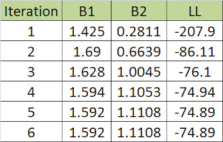
After simulating the data and running the procedure, the algorithm converges in 6 steps, (i.e. the solutions for the β estimates are reached in 6steps). Below is summary of the results:
Also, plotting these via PROC G3D, (with my crude annotations) shows how with each step or iteration of the algoritm, we get closer and closer to maximiizing the log of the likelihood function.



And we specify a likelihood function based on the normal density:

(Intercept) 1.9910 0.1961 10.156 < 2e-16 ***
X[, 2] 2.9102 0.3418 8.514 2.01e-13 ***
---
Signif. codes: 0 ‘***’ 0.001 ‘**’ 0.01 ‘*’ 0.05 ‘.’ 0.1 ‘ ’ 1
F-statistic: 72.48 on 1 and 98 DF, p-value: 2.009e-13

Created by Pretty R at inside-R.org
I recently found some notes posted for a biostatistics course at the University of Minnesota, (I believe it was taught by John Connet) which presented SAS code for implementing maximum likelihood estimation using Newton's method via PROC IML. As noted in my post on logistic regression:
When we undertake MLE we typically maximize the log of the likelihood function as follows:
Max Log(L(β)) or LL ‘log likelihood’ or solve:
∂Log(L(β))/∂β = 0
As noted in the biostats course notes, typically we can't solve for these formulas directly, but the solutions have to be estimated iteratively. One method of doing this is Netwon's Method, which the IML code implements. (see SAS code that follows below)
After simulating the data and running the procedure, the algorithm converges in 6 steps, (i.e. the solutions for the β estimates are reached in 6steps). Below is summary of the results:

Also, plotting these via PROC G3D, (with my crude annotations) shows how with each step or iteration of the algoritm, we get closer and closer to maximiizing the log of the likelihood function.

Note, running PROC LOGISTIC (which actually implements Fisher Scoring) against the simulated data gives very similar results to the algorithm implemented in PROC IML:

Note, given certain assumptions, you can get similar results from implementing least squares and maximum likelihood. If we make the following assumptions:


Maximizing this with respect to the β 's will give the same least squares results.
Using R (code below) I simulated data and specified the likelihood function above for a single variable regression. (for more info see Ajay Shah's notes , as well as Maximum Likelihood Programming in R)
Running a regression on the simulated data (using R's 'lm' operation) produced the following results:
Coefficients:
Estimate Std. Error t value Pr(>|t|) (Intercept) 1.9910 0.1961 10.156 < 2e-16 ***
X[, 2] 2.9102 0.3418 8.514 2.01e-13 ***
---
Signif. codes: 0 ‘***’ 0.001 ‘**’ 0.01 ‘*’ 0.05 ‘.’ 0.1 ‘ ’ 1
Residual standard error: 0.9693 on 98 degrees of freedom
Multiple R-squared: 0.4252, Adjusted R-squared: 0.4193 F-statistic: 72.48 on 1 and 98 DF, p-value: 2.009e-13
The 'beta' coefficeint on x is 2.9102 . Using the R function 'optim' I optimized the likelihood function, getting the results below, which are on par with the actual regression I just ran above:
$par
[1] 1.9910299 2.9101836 0.9207324
In order B0 = 1.9910299 and B1 = 2.9101836 which are the results we got before.
Iterating values for B1 and using the R 'apply' function in conjunction with the specified likelihood function, I plotted the values of the likelihood function for each iterated value of B1. As shown, the likelihood function is maximized at B1 ~ 2.9101836

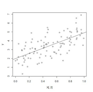
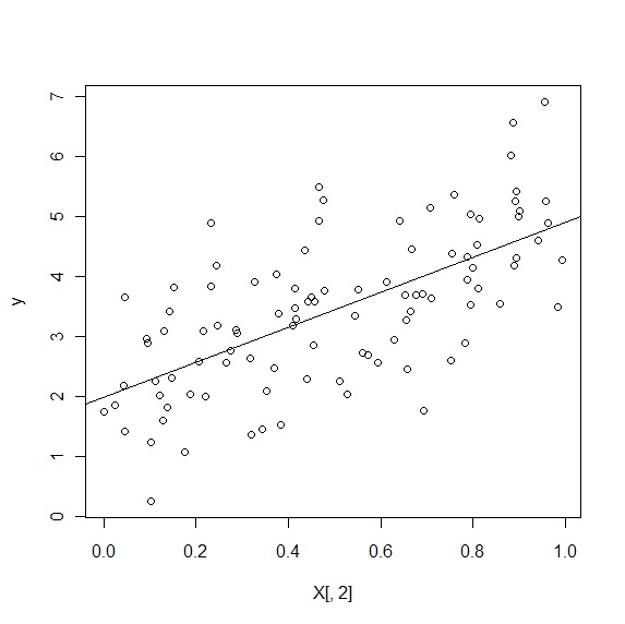
And below is the OLS line (with the same beta's we get from maximum likelihood above) plotted against the simulated data:
SAS Code Below:
/* PROC IML MLE SIMULATION */
/* Program to compute maximum likelihood estimates .... */;
/* Based on Newton-Raphson methods - uses IML */;
footnote "program: /home/walleye/john-c/5421/imlml.sas &sysdate &systime" ;
options linesize = 80 ;
data sim ;
one = 1 ;
a = 2 ;
b = 1 ;
n = 300 ;
seed = 20000214 ;
/* Simulated data from logistic distribution */;
do i = 1 to n ;
u = 2 * i / n ;
p = 1 / (1 + exp(-a - b * u)) ;
r = ranuni(seed) ;
yi = 0 ;
if r lt p then yi = 1 ;
output ;
end ;
run ;
/*look at data */
proc univariate data = sim;
var p;
histogram p;
run;
/* Logistic analysis of simulated data ...... */;
proc logistic descending data = sim outmodel = logit;
model yi = u / lackfit rsq;
score data =sim out= score1 fitstat ;
title1 'Proc logistic results ... ' ;
run ;
/* Begin proc iml .............................. */;
title1 'PROC IML Results ...' ;
proc iml ;
use sim ; /* Input the simulated dataset */;
read all var {one u} into x ; /* Read the design matrix into x */;
read all var {yi} into y ; /* Read the outcome data into y */;
p = 2 ; /* Set the number of parameters */;
beta = {0.00, 0.00} ; /* Initialize the param. vector */;
/* -------------------------------------------------------------------*/;
/* Module which computes loglikelihood and derivatives ... */;
start loglike(beta, p, x, y, l, dl, d2l) ;
n = 300 ;
l = 0 ; /* Initialize log likelihood ... */;
dl = j(p, 1, 0) ; /* Initialize 1st derivatives... */;
d2l = j(p, p, 0) ; /* Initialize 2nd derivatives... */;
do i = 1 to n ;
xi = x[i,] ;
yi = y[i] ;
xibeta = xi * beta ;
w = exp(-xibeta) ;
/* The log likelihood for the i-th observation ... */;
iloglike = log((1 - yi) * w + yi) - log(1 + w) ;
l = l + iloglike ;
do j = 1 to p ;
xij = xi[j] ;
/* The jth 1st derivative of the log likelihood for the ith obs */;
jdlogl = -(1 - yi) * w * xij / ((1 - yi) * w + yi)
+ w * xij / (1 + w) ;
dtemp = dl[j] + jdlogl ;
dl[j] = dtemp ;
do k = 1 to p ;
xik = xi[k] ;
/* The jkth 2nd derivative of the log likelihood for the ith obs */;
jkd2logl = ((1 - yi) * w * xij * xik * ((1 - yi) * w + yi)
-(1 - yi) * w * xij * ((1 - yi) * w * xik))/
((1 - yi) * w + yi)**2
+ (-w * xij * xik * (1 + w) + w * w * xij * xik)/
(1 + w)**2 ;
d2temp = d2l[j, k] ;
d2l[j, k] = d2temp + jkd2logl ;
end ;
end ;
end ;
finish loglike ;
/* -------------------------------------------------------------------*/;
eps = 1e-8 ;
diff = 1 ;
/* The following do loop stops when the increments in beta are */;
/* sufficiently small, or when number of iterations reaches 20 */;
do iter = 1 to 20 while(diff > eps) ;
run loglike(beta, p, x, y, l, dl, d2l) ;
invd2l = inv(d2l) ;
beta = beta - invd2l * dl ; /* The key Newton step ... */;
diff = max(abs(invd2l * dl)) ;
print iter l dl d2l diff beta ;
end ;
b1 = beta[1] ;
b2 = beta[2] ;
serr1 = sqrt(-invd2l[1, 1]) ;
serr2 = sqrt(-invd2l[2, 2]) ;
covar = -invd2l ;
llratio = - 2 * l ;
print ' -2 * loglikelihood = ' llratio ;
print 'b1 coeff, std err : ' b1 serr1 ;
print 'b2 coeff, std err : ' b2 serr2 ;
print 'covariance matrix : ' covar ;
quit ;
/* read the values of LL and beta's into a SAS data set*/
data ldat;
input B1 B2 LL;
cards;
1.424660 0.2810698 -207.90000
1.689885 0.6639477 -86.11339
1.628445 1.0044749 -76.10077
1.593570 1.1053311 -74.93779
1.591699 1.1108087 -74.89053
1.591694 1.1108238 -74.89040
;
run;
PROC G3D DATA=ldat GOUT=THECAT;
SCAT B1 * B2 = LL / GRID SIZE=1 COLOR='GREEN' XTICKNUM =10 YTICKNUM =10;
TITLE'';
RUN; QUIT;
R Code Below:
# *------------------------------------------------------------------
# | PROGRAM NAME: mle_sim
# | DATE: 5/15/11
# | CREATED BY:  Matt Bogard
# | PROJECT FILE:  econometric sense
# *----------------------------------------------------------------
# | PURPOSE: demonstrate mle in R
# |
# *------------------------------------------------------------------
# | COMMENTS:
# |
# |  1: see also: Maximum Likelihood Programming in R Marco R. Steenbergen
# |       http://www.artsci.wustl.edu/~jmonogan/computing/r/MLE_in_R.pdf
# |  2: notes from: Ajay Sha -'Roll Your Own Likelihood Function in R here: http://www.mayin.org/ajayshah/KB/R/documents/mle/mle.html
# |  3: Ajay also has lots of other R by example links here: http://www.mayin.org/ajayshah/KB/R/
# |*------------------------------------------------------------------
#


# simulate data for x
set.seed(123)

X<-cbind(1,runif(100))
dim(X)


# set true values for the betas and variance

theta.true<-c(2,3,1) # B0, B1, sigma^2

# generate  y-values

y<-X%*%theta.true[1:2] + rnorm(100)
dim(y)

plot(y~X[,2])


# specify the likelihood function based on the standard normal distribution

ols.lf<-function(theta,y,X){ n<-nrow(X)
k<-ncol(X)
beta<-theta[1:k]
sigma2<-theta[k+1]
e<-y-X%*%beta
logl<- -.5*n*log(2*pi)-.5*n*log(sigma2)-
((t(e)%*%e)/(2*sigma2))
return(-logl)
}


# optimize the likelihood function with initial values for BO, B1, sigma^2 -> 1,1,1

p<-optim(c(1,1,1),ols.lf,method="BFGS",hessian=T,y=y,X=X)

names(p)

print(p)


# note SE(B) =  square root of the diagonals of the inverse of the hession

OI<-solve(p$hessian)

se<-sqrt(diag(OI))


# compare to linear model

d<-summary(lm(y~X[,2]))


# plotting

theta.ols <- c(sigma2 = d$sigma^2, d$coefficients[,1])  # get linear model betas from output
theta <- theta.ols  # theta for next simulation
delta.values <- seq(-1.5, 1.5, .01)  # iterate beta values by amounts between -1.5 and 1.5

logl.values <- as.numeric(lapply(delta.values,
                                 function(x) {-ols.lf(theta+c(0,0,x),y,X)}))  # this produces log likelihood values for values of X,y,and iterated beta's

#  plot likelihood function and betas
plot(theta[3]+delta.values, logl.values, type="l", lwd=3, col="blue",
     xlab="B1", ylab="Log likelihood")
Subscribe to:
Posts (Atom)